$$ 0 = \left\{\delta \mathbf {U} \right\} ^ {T} \left(\left[ \mathbf {K} _ {N L} \right] + \left[ \mathbf {K} _ {L} \right]\right) \left\{\Delta \mathbf {U} \right\} - \left\{\delta \mathbf {U} \right\} ^ {T} \left(\left\{\mathbf {Q} _ {T} \right\} + \left\{\mathbf {Q} _ {B} \right\} - \left\{\mathbf {F} \right\}\right) \tag {2.46} $$ 이때 δU 는 임의의 값이므로 식(2.46)을 만족하기 위해서는 식(2.47)과 같이 쓸 수 있고, 식(2.47)은 Newton-Raphson 형식으로 ΔU 에 대한 반복 계산을 통해 수렴값을 찾아 나감으로써 비선형 해석을 수행할 수 있다. $$ \left(\left[ \mathbf {K} _ {N L} \right] + \left[ \mathbf {K} _ {L} \right]\right) \left\{\Delta \mathbf {U} \right\} = \left\{\mathbf {Q} _ {T} \right\} + \left\{\mathbf {Q} _ {B} \right\} - \left\{\mathbf {F} \right\} \tag {2.47} $$ 여기서 $K_{NL}$ 과 $K_{L}$ 의 합이 기울기 강성 행렬(tangent stiffness matrix)이 된다. # 2.2.1 Finite Rotation Formulation 셀의 형상이 변함에 따라 각각의 노드에서 정의 된 벡터 $\left(\mathbf{V}^{1}, \mathbf{V}^{2}, \mathbf{V}^{n}\right)$ 역시 시간에 따라 변하게 된다. 즉 시간에 따른 회전각 $\alpha, \beta$ 의 변화에 따라 $\mathbf{V}^{n}$ 이 변하고, 또한 그에 따라 $\mathbf{V}^{1}$ 과 $\mathbf{V}^{2}$ 도 변하게 된다. 이를 관계식으로 표현하면, 식(2.48)과 같이 쓸 수 있다. $$ { } ^ { t + \Delta t } \mathbf { V } _ { I } ^ { n } = { } _ { t } ^ { t + \Delta t } \mathbf { R } _ { I } \cdot { } ^ { t } \mathbf { V } _ { I } ^ { n } \tag {2.48} $$ 식(2.48)은 시간이 t부터 $t+\Delta t$ 까지 변할 때 노드 I에서의 법선 벡터의 변화를 보여주는 식으로 ${}^{t+\Delta t}_{t}R_{I}$ 는 회전 텐서(rotation tensor)를 의미하며, $\left\|^{t}V_{I}^{n}\right\|=\left\|^{t+\Delta t}V_{I}^{n}\right\|=1$ 이다. [9] 그리고 회전 텐서 $^{t+\Delta t}_{t}R_{I}$ 은 $V^{1}, V^{2}, V^{n}$ 을 정규직교 기저(orthonormal basis)로 하는 좌표계에서 식(2.49)와 같이 행렬 형태로 나타낼 수 있다. [10] $$ \left[ \begin{array}{l} t + \Delta t \\ t \end{array} R _ {I} \right] = \left[ \mathbf {1} _ {3} \right] + \frac {\sin \left(\widetilde {\theta} _ {I}\right)}{\widetilde {\theta} _ {I}} \left[ \Theta_ {I} \right] + \frac {1}{2} \left[ \frac {\sin \left(\frac {\widetilde {\theta} _ {I}}{2}\right)}{\left(\frac {\widetilde {\theta} _ {I}}{2}\right)} \right] ^ {2} \left[ \Theta_ {I} \right] ^ {2} \tag {2.49} $$ 이 때 $\left[1_{3}\right]$ 은 3행 3열의 단위 행렬을 의미하며, $\widetilde{\theta}_{I}$ 와 $\left[\Theta_{I}\right]$ 는 각각식(2.50), (2.51)과 같이 나타낼 수 있다. $$ \widetilde {\theta} _ {I} = \left[ \left(\alpha_ {I}\right) ^ {2} + \left(\beta_ {I}\right) ^ {2} \right] ^ {\frac {1}{2}} \tag {2.50} $$ $$ \left[ \Theta_ {I} \right] = \left[ \begin{array}{c c c} 0 & 0 & \beta_ {I} \\ 0 & 0 & - \alpha_ {I} \\ - \beta_ {I} & \alpha_ {I} & 0 \end{array} \right] \tag {2.51} $$ 여기서 $\alpha_{I}$ 와 $\beta_{I}$ 가 미소 증분 회전(infinitesimal incremental rotation)이면, 각각 $V^{1}$ , $V^{2}$ 에 대한 독립적인 미소 회전(independent infinitesimal rotation)을 의미하고, $\alpha_{I}$ 와 $\beta_{I}$ 가 유한 증분 회전(finite incremental rotation)이면, $\alpha_{I}$ 와 $\beta_{I}$ 는 서로 독립적이지 않으며 회전 텐서를 정의하는 변수가 된다. [9] # 2.2.2 Constitutive Matrix 구성 행렬(constitutive matrix)의 경우 평면응력(plane stress) 가정을 사용하였으며, 식(2.52)와 같다. 이 때 $\kappa$ 는 전단 보정 계수(shear correction factor)로 5/6를 사용하였다. 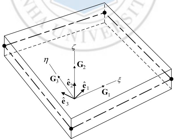$$ \left[ \widetilde {D} \right] _ {x y z} = \frac {E}{1 - \nu^ {2}} \left[ \begin{array}{c c c c c c} 1 & \nu & 0 & 0 & 0 & 0 \\ \nu & 1 & 0 & 0 & 0 & 0 \\ 0 & 0 & 0 & 0 & 0 & 0 \\ 0 & 0 & 0 & \kappa \frac {1 - \nu}{2} & 0 & 0 \\ 0 & 0 & 0 & 0 & \kappa \frac {1 - \nu}{2} & 0 \\ 0 & 0 & 0 & 0 & 0 & \frac {1 - \nu}{2} \end{array} \right] \tag {2.52} $$ 하지만 식(2.52)의 경우 지역 직교 좌표계(local Cartesian coordinate system)에서 정의되므로 이를 고유 좌표계(natural coordinate system)에서 정의하기 위해서는 변환 행렬(transformation matrix)을 사용해야 한다. 지역 직교 좌표계와 고유 좌표계 사이의 관계는 Fig. 4와 같으며, 여기서 $G_{1}, G_{2}, G_{3}$ 는 고유 좌표계의 콩변 기저(covariant basis)이고, $\hat{e}_{1}, \hat{e}_{2}, \hat{e}_{3}$ 는 지역 직교 좌표계의 기저를 의미한다. 

text_image

η G₃ ê₂ ê₁ ê₃ G₂ ξ G₁

Fig. 4 Local Cartesian coordinate system 변형률과 응력에 대한 좌표변환은 식(2.53), (2.54)와 같으며, 이로부터 구성 행렬의 좌표변환은 식(2.55)와 같이 나타낼 수 있다. 여기서 $\widetilde{E}$ , $\widetilde{S}$ , $\widetilde{D}$ 와 E, S, D는 각각 지역 직교 좌표계와 고유 좌표계에서의 변형률, 응력, 구성 행렬을 의미한다. 그리고 $\left[T\right]_{\xi \rightarrow x}$ 는 고유 좌표계에서 정의된 값을 지역 직교 좌표계로 변환해주는 변환 행렬이다. $$ \left\{\widetilde {E} \right\} _ {x y z} = [ T ] _ {\xi \rightarrow x} \left\{E \right\} _ {\xi \eta \zeta} \tag {2.53} $$ $$ \begin{array}{l} \left\{S \right\} _ {\xi \eta \zeta} = \left[ T \right] _ {x \rightarrow \xi} \left\{\widetilde {S} \right\} _ {x y z} = \left[ T \right] _ {\xi \rightarrow x} ^ {T} \left[ \widetilde {D} \right] _ {x y z} \left\{\widetilde {E} \right\} _ {x y z} \tag {2.54} \\ = \left[ T \right] _ {\xi \rightarrow x} ^ {T} \left[ \widetilde {D} \right] _ {x y z} \left[ T \right] _ {\xi \rightarrow x} \left\{E \right\} _ {\xi \eta \zeta} = \left[ D \right] _ {\xi \eta \zeta} \left\{E \right\} _ {\xi \eta \zeta} \\ \end{array} $$ $$ \left[ D \right] _ {\xi \eta \zeta} = \left[ T \right] _ {\xi \rightarrow x} ^ {T} \left[ \widetilde {D} \right] _ {x y z} \left[ T \right] _ {\xi \rightarrow x} \tag {2.55} $$ 이 때 $[T]_{\xi \rightarrow x}$ 는 식(2.56)과 같이 나타낼 수 있고, 각각의 성분은 식(2.57)과 같다. $$ \left[ T \right] _ {\xi \rightarrow x} = \left[\begin{array}{c c c c c c c}a _ {1} a _ {1}&b _ {1} b _ {1}&c _ {1} c _ {1}&b _ {1} c _ {1}&a _ {1} c _ {1}&a _ {1} b _ {1}\\a _ {2} a _ {2}&b _ {2} b _ {2}&c _ {2} c _ {2}&b _ {2} c _ {2}&a _ {2} c _ {2}&a _ {2} b _ {2}\\a _ {3} a _ {3}&b _ {3} b _ {3}&c _ {3} c _ {3}&b _ {3} c _ {3}&a _ {3} c _ {3}&a _ {3} b _ {3}\\2 a _ {2} a _ {3}&2 b _ {2} b _ {3}&2 c _ {2} c _ {3}&b _ {2} c _ {3} + c _ {2} b _ {3}&a _ {2} c _ {3} + c _ {2} a _ {3}&a _ {2} b _ {3} + b _ {2} a _ {3}\\2 a _ {1} a _ {3}&2 b _ {1} b _ {3}&2 c _ {1} c _ {3}&b _ {1} c _ {3} + c _ {1} b _ {3}&a _ {1} c _ {3} + c _ {1} a _ {3}&a _ {1} b _ {3} + b _ {1} a _ {3}\\2 a _ {1} a _ {2}&2 b _ {1} b _ {2}&2 c _ {1} c _ {2}&b _ {1} c _ {2} + c _ {1} b _ {2}&a _ {1} c _ {2} + c _ {1} a _ {2}&a _ {1} b _ {2} + b _ {1} a _ {2}\end{array}\right] \tag {2.56} $$ $$ a _ {1} = \mathbf {r} _ {1} \cdot \mathbf {G} ^ {1} \quad b _ {1} = \mathbf {r} _ {1} \cdot \mathbf {G} ^ {2} \quad c _ {1} = \mathbf {r} _ {1} \cdot \mathbf {G} ^ {3} $$ $$ a _ {2} = \mathbf {r} _ {2} \cdot \mathbf {G} ^ {1} \quad b _ {2} = \mathbf {r} _ {2} \cdot \mathbf {G} ^ {2} \quad c _ {2} = \mathbf {r} _ {2} \cdot \mathbf {G} ^ {3} \tag {2.57} $$ $$ a _ {3} = \mathbf {r} _ {3} \cdot \mathbf {G} ^ {1} \quad b _ {3} = \mathbf {r} _ {3} \cdot \mathbf {G} ^ {2} \quad c _ {3} = \mathbf {r} _ {3} \cdot \mathbf {G} ^ {3} $$ 그리고 지역 직교 좌표계의 기저 $\hat{\mathbf{e}}_{1}, \hat{\mathbf{e}}_{2}, \hat{\mathbf{e}}_{3}$ 는 식(2.58)와 같이 고유 좌표계의 공변 기저(covariant basis) $\mathbf{G}_{1}, \mathbf{G}_{2}, \mathbf{G}_{3}$ 로부터 구할 수 있다. $$ \hat {\mathbf {e}} _ {3} = \frac {\mathbf {G} _ {3}}{\left\| \mathbf {G} _ {3} \right\|}, \quad \hat {\mathbf {e}} _ {1} = \frac {\mathbf {G} _ {2} \times \hat {\mathbf {e}} _ {3}}{\left\| \mathbf {G} _ {2} \times \hat {\mathbf {e}} _ {3} \right\|}, \quad \hat {\mathbf {e}} _ {2} = \hat {\mathbf {e}} _ {3} \times \hat {\mathbf {e}} _ {1} \tag {2.58} $$ # 2.2.3 Mass Matrix 질량 행렬(mass matrix)은 물체 내에 연속적으로 분포되어 있는 물체의질량을 요소망 내 각 절점(node)에 집중 질량(lumped mass) 형식으로이산화시켜 놓은 것으로, 이 질량 행렬 내 각 행렬요소를 합하면, 물체의전체 질량과 같게 되며, 물체의 자중, 운동량, 관성력을 표현한다. 진동 및 동적 좌굴 해석을 하기 위해서는 이러한 질량 행렬이필요하며, 일반적으로 일관 질량 행렬(consistent mass matrix)과 집중 질량행렬(lumped mass matrix)있다. 일관 질량 행렬은 식(2.59)와 같이 나타낼수 있다.[2] 여기서 는 밀도, N은 형상 함수 행렬을 나타낸다. $$ \left[ \widetilde {\mathbf {M}} \right] = \int_ {V} \rho [ \mathbf {N} ] ^ {T} [ \mathbf {N} ] d V \tag {2.59} $$ 집중 질량 행렬의 경우 일관 질량 행렬을 대각화(diagonalization)함으로써 연산에 필요한 용량과 연산 시간을 줄일 수 있다는 장점이있지만[2] 본 논문에서는 물체의 강성을 줄임으로써 유연한 결과를 얻기위해 집중 질량 행렬을 사용하였다. 일관 질량 행렬을 대각화하는방법에는 다양한 방법들이 존재하며, 본 논문에서는 각각의 행을 합하는방법(row-sum technique)을 사용하였다.[3] 식(2.60)으로부터 각각의 요소에대한 일관 질량 행렬 M\~ 의 행의 합을 구한다. 그리고 이를 식(2.61)과같이 새로운 집중 질량 행렬 M 의 대각항(diagonal entries)에 대입하고,비대각항(off-diagonal entries)은 영(零)을 대입한다. 이 때 n은 요소의절점의 개수와 자유도의 곱을 나타낸다. 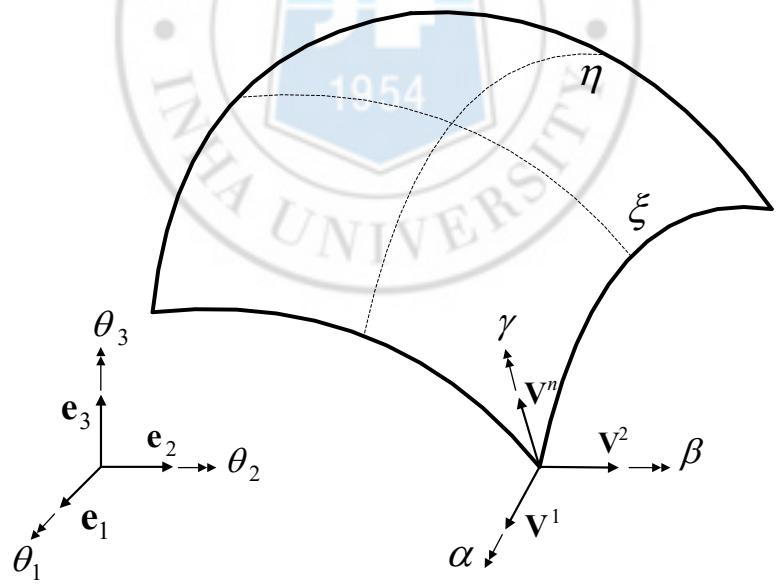$$ S (i) = \sum_ {j = 1} ^ {n} \widetilde {\mathbf {M}} (i, j) \quad \text { for } i = 1, n \tag {2.60} $$ $$ \mathbf {M} (i, j) = S (i) \quad \text {for} i = 1, n \tag {2.61} $$ $$ \mathbf {M} (i, j) = 0 \quad \text { for } i \neq j $$ # 2.2.4 6-DOF Shell Element 일반적으로 셀 요소는 5개의 자유도(degree of freedom)를 사용하며, 법선 벡터(normal vector)는 각 절점당 하나의 법선 벡터를 갖는다. 하지만 셀 요소를 보강재(stiffener)로 사용하는 경우, 셀 요소와 셀 요소의 결합을 위해서는 6개의 자유도가 필요하며, 이와 더불어 각 절점에서 정의되는 법선 벡터에 대한 구속 조건이 필요하다. 이에 본 논문에서는 각 절점에서 정의되는 지역 좌표계(local coordinate system)를 전역 직교 좌표계(global Cartesian coordinate system)로 변환해 줌으로써 셀 요소와 셀 요소의 결합을 구성하였다. 이 때 지역 좌표계는 $V^{1}$ , $V^{2}$ , $V^{n}$ 을 기저로 하는 좌표계로 표현된다. 전역 직교 좌표계에서 정의되는 회전 자유도 $\theta_{1}, \theta_{2}, \theta_{3}$ 와 지역 좌표계에 의해 정의되는 회전 자유도 $\alpha, \beta, \gamma$ 는 식(2.62)와 같은 관계식을 만족해야 한다. 

text_image

1954 INIA UNIVERSITY η ξ γ Vⁿ V² β α θ₁ θ₂ e₁ e₂ e₃ θ₃ e₃

Fig. 5 Global Cartesian coordinate system and local coordinate system $$ \theta_ {1} \mathbf {e} _ {1} + \theta_ {2} \mathbf {e} _ {2} + \theta_ {3} \mathbf {e} _ {3} = \alpha \mathbf {V} ^ {1} + \beta \mathbf {V} ^ {2} + \gamma \mathbf {V} ^ {n} \tag {2.62} $$ 이 때 식(2.62)의 좌변과 우변에 각각 벡터 $V^{1}$ 을 곱해주면, 식(2.63)과 같이 나타낼 수 있고, 마찬가지 방법으로 $V^{2}$ , $V^{n}$ 을 곱해주면, 각각 식(2.64), (2.65)와 같이 나타낼 수 있다. $$ \alpha = \theta_ {1} \left(\mathbf {e} _ {1} \cdot \mathbf {V} ^ {1}\right) + \theta_ {2} \left(\mathbf {e} _ {2} \cdot \mathbf {V} ^ {1}\right) + \theta_ {3} \left(\mathbf {e} _ {3} \cdot \mathbf {V} ^ {1}\right) \tag {2.63} $$ $$ \beta = \theta_ {1} \left(\mathbf {e} _ {1} \cdot \mathbf {V} ^ {2}\right) + \theta_ {2} \left(\mathbf {e} _ {2} \cdot \mathbf {V} ^ {2}\right) + \theta_ {3} \left(\mathbf {e} _ {3} \cdot \mathbf {V} ^ {2}\right) \tag {2.64} $$ $$ \gamma = \theta_ {1} \left(\mathbf {e} _ {1} \cdot \mathbf {V} ^ {n}\right) + \theta_ {2} \left(\mathbf {e} _ {2} \cdot \mathbf {V} ^ {n}\right) + \theta_ {3} \left(\mathbf {e} _ {3} \cdot \mathbf {V} ^ {n}\right) \tag {2.65} $$ 이를 행렬 형태로 표현해 주면 식(2.66)과 같이 쓸 수 있다. $$ \left\{ \begin{array}{l} \alpha \\ \beta \\ \gamma \end{array} \right\} = \left[ \begin{array}{l} \left(\mathbf {e} _ {1} \cdot \mathbf {V} ^ {1}\right) \left(\mathbf {e} _ {2} \cdot \mathbf {V} ^ {1}\right) \left(\mathbf {e} _ {3} \cdot \mathbf {V} ^ {1}\right) \\ \left(\mathbf {e} _ {1} \cdot \mathbf {V} ^ {2}\right) \left(\mathbf {e} _ {2} \cdot \mathbf {V} ^ {2}\right) \left(\mathbf {e} _ {3} \cdot \mathbf {V} ^ {2}\right) \\ \left(\mathbf {e} _ {1} \cdot \mathbf {V} ^ {n}\right) \left(\mathbf {e} _ {2} \cdot \mathbf {V} ^ {n}\right) \left(\mathbf {e} _ {3} \cdot \mathbf {V} ^ {n}\right) \end{array} \right] \left\{ \begin{array}{l} \theta_ {1} \\ \theta_ {2} \\ \theta_ {3} \end{array} \right\} \tag {2.66} $$ 위 식으로부터 전역 직교 좌표계에서 지역 좌표계로 변환해 주는 행렬은 식(2.67)과 같이 정의 할 수 있으며, 이 때 L 은 식(2.68)과 같다. [5] $$ \left[ \widetilde {T} \right] = \left[ \begin{array}{c c c c c c} \mathbf {1} _ {3} & 0 & 0 & \dots & 0 & 0 \\ & \mathbf {L} & 0 & & & 0 \\ & & \ddots & \ddots & & \vdots \\ & & & \ddots & 0 & 0 \\ & \text {sym.} & & & \mathbf {1} _ {3} & 0 \\ & & & & & \mathbf {L} \end{array} \right] \tag {2.67} $$ $$ [ \mathbf {L} ] = \left[ \begin{array}{l} \left(\mathbf {e} _ {1} \cdot \mathbf {V} ^ {1}\right) \left(\mathbf {e} _ {2} \cdot \mathbf {V} ^ {1}\right) \left(\mathbf {e} _ {3} \cdot \mathbf {V} ^ {1}\right) \\ \left(\mathbf {e} _ {1} \cdot \mathbf {V} ^ {2}\right) \left(\mathbf {e} _ {2} \cdot \mathbf {V} ^ {2}\right) \left(\mathbf {e} _ {3} \cdot \mathbf {V} ^ {2}\right) \\ \left(\mathbf {e} _ {1} \cdot \mathbf {V} ^ {n}\right) \left(\mathbf {e} _ {2} \cdot \mathbf {V} ^ {n}\right) \left(\mathbf {e} _ {3} \cdot \mathbf {V} ^ {n}\right) \end{array} \right] \tag {2.68} $$ 만약 변위 벡터와 힘 벡터를 전역 좌표계에서 지역 좌표계로 변환해주면 각각 식(2.69), (2.70)과 같이 나타낼 수 있다. 이 때 위 첨자 e는 요소에 대해 정의 되었음을 의미한다.[4] $$ \{\widetilde {\mathbf {u}} \} ^ {e} = \left[ \widetilde {T} \right] \{\mathbf {u} \} ^ {e} \tag {2.69} $$ $$ \left\{\widetilde {\mathbf {f}} \right\} ^ {e} = \left[ \widetilde {T} \right] \left\{\mathbf {f} \right\} ^ {e} \tag {2.70} $$ 그리고 강성 행렬(stiffness matrix)은 지역 좌표계에서 식(2.71)과 같은 선형 관계식으로 나타낼 수 있다.[4] $$ \left\{\widetilde {\mathbf {f}} \right\} ^ {e} = \left[ \widetilde {\mathbf {K}} \right] ^ {e} \left\{\widetilde {\mathbf {u}} \right\} ^ {e} \tag {2.71} $$ 여기서 식(2.69)와 (2.70)을 식(2.71)에 대입해주면, 식(2.72)와 같이 나타낼 수 있고, 따라서 강성 행렬을 지역 좌표계에서 전역 좌표계로 변환해주는 관계식은 식(2.73)과 같다. [4] $$ \left\{\mathbf {f} \right\} ^ {e} = \left[ \widetilde {T} \right] ^ {T} \left[ \widetilde {\mathbf {K}} \right] ^ {e} \left[ \widetilde {T} \right] \left\{\mathbf {u} \right\} ^ {e} \tag {2.72} $$ $$ \left[ \mathbf {K} \right] ^ {e} = \left[ \widetilde {T} \right] ^ {T} \left[ \widetilde {\mathbf {K}} \right] ^ {e} \left[ \widetilde {T} \right] \tag {2.73} $$ 하지만 6-자유도의 도입으로 강성 행렬 $\tilde{\mathbf{K}}^{e}$ 의 경우 여섯 번째 자유도에 해당하는 행과 열이 모두 영(雫)이 되고, 이로 인해 특이점(singularity)이 발생하게 된다. 이에 본 논문에서는 이를 방지하기 위해서 여섯 번째 자유도의 대각항(diagonal entries)에 식(2.75)와 같이 대각항 최소값의 $10^{-3}$ 비율을 갖는 값을 대입하였다. $$ \left[ \widetilde {\mathbf {K}} \right] ^ {e} = \left[ \begin{array}{c c c c c c c c c c c c c c c c} & & & & & 0 & & & & & & & & & 0 \\ & & & & & 0 & & & & & & & & & 0 \\ & & \mathbf {K} _ {1} & & & 0 & & & & \mathbf {K} _ {2} & & & & 0 \\ & & & & & 0 & & & & & & & & 0 \\ & & & & & 0 & & & & & & & & 0 \\ 0 & 0 & 0 & 0 & 0 & d & \dots & \dots & 0 & 0 & 0 & 0 & 0 & 0 \\ & & & & & \vdots & \ddots & & & & & & & \vdots \\ & & & & & \vdots & & \ddots & & & & & & \vdots \\ & & & & & 0 & & & & & & & & 0 \\ & & & & & 0 & & & & & & & & 0 \\ & & \mathbf {K} _ {3} & & & 0 & & & & \mathbf {K} _ {4} & & & 0 \\ & & & & & 0 & & & & & & & & 0 \\ & & & & & 0 & & & & & & & & 0 \\ 0 & 0 & 0 & 0 & 0 & 0 & \dots & \dots & 0 & 0 & 0 & 0 & 0 & d \end{array} \right] \tag {2.74} $$ $$ d = \min \left(\widetilde {\mathbf {K}} ^ {e} (i, i)\right) \times 1 0 ^ {- 3} \quad \text { for } i = 1, n \tag {2.75} $$ 그리고 6-자유도의 도입으로 회전 텐서를 구하는데 필요한 식(2.50)과 (2.51)은 식(2.76), (2.77)과 같은 형태가 된다. $$ \widetilde {\theta} _ {I} = \left[ \left(\alpha_ {I}\right) ^ {2} + \left(\beta_ {I}\right) ^ {2} + \left(\gamma_ {I}\right) ^ {2} \right] ^ {\frac {1}{2}} \tag {2.76} $$ $$ \left[ \Theta_ {I} \right] = \left[ \begin{array}{c c c} 0 & - \gamma_ {I} & \beta_ {I} \\ \gamma_ {I} & 0 & - \alpha_ {I} \\ - \beta_ {I} & \alpha_ {I} & 0 \end{array} \right] \tag {2.77} $$ # 2.3 Buckling Theory 가느다란 기둥을 축 방향으로 누르거나 얇은 판을 판과 평행한방향으로 압축하면, 하중이 어느 크기에 도달하는 순간 갑자기 판이 횡방향으로 과도하게 휘어지는 축 방향 변위(lateral displacement)가 발생한다.물체의 이러한 거동을 좌굴 혹은 붕괴라고 정의하며 구조물의 안전성에치명적인 문제점을 야기시킨다. 좌굴이 발생하기 전까지 물체는 정적인 평형상태를 유지하지만, 일단좌굴이 발생하면 평형상태가 깨어지고 횡 방향으로 큰 변형이 발생하여외부 하중을 더 이상 지탱할 수 없게 된다. 이러한 좌굴은 비단 가느다란기둥이나 얇은 판의 휨 좌굴(flexural buckling)에만 국한되는 것이 아니며,물체의 국부 영역에 지역적으로 발생하는 국부 좌굴(local buckling),전단력에 의하여 야기되는 전단 좌굴(shear buckling) 그리고 비틀림에의해 발생하는 비틀림 좌굴(torsion buckling) 등이 있다. 한편 좌굴에 의한 물체의 변형이 구조물이 이루는 평면 내에 있느냐아니면 바깥에 있느냐에 따라 면내 좌굴(in-plane buckling) 그리고 면외좌굴(out of plane buckling)로 구분하기도 한다. 좌굴은 거의 대부분 물체의형상이나 하중 조건의 불완전성(imperfection)에 기인한다. 예를 들어,기둥의 단면 중심에 정확히 축 방향으로 집중 압축력을 가한다고 했을때, 이론적으로는 횡 방향으로 휨을 발생시킬 하중이나 모멘트 성분이전혀 없기 때문에 좌굴이 발생해서는 안 된다. 하지만 실제 기둥은 정확히 원형 단면이 아닐 뿐만 아니라 압축력이작용하는 지점도 정확히 축의 중심에 위치하지 않는다. 따라서기하학적인 불완전성과 축 중심에서 어느 정도 편심된 위치에 압축력이작용함에 따른 불완전함에 따라 횡 방향으로의 변위가 발생하게 된다. 좌굴은 물체의 가느다란 정도를 나타내는 형상 종횡비(aspect ratio)가클수록 보다 쉽게 발생한다. 다시 말해 길이가 긴 기둥이 짧은 기둥에비해 좌굴이 보다 쉽게 발생한다. 그리고 좌굴은 동일한 재질, 형상 및하중조건에서도 물체를 구속하는 경계조건(boundary condition)에 크게영향을 받는다. 또한 좌굴은 작용하는 힘이 정적 하중이냐 동적 하중이냐에 따라 정적