Here we present the principle of minimum potential energy as used to derive the spring element equations. We will illustrate this concept by applying it to the simplest of elements in hopes that the reader will then be more comfortable when applying it to handle more complicated element types in subsequent chapters. The total potential energy $\pi _ { p }$ of a structure is expressed in terms of displacements. In the finite element formulation, these will generally be nodal displacements such that $\pi _ { p } = \pi _ { p } ( d _ { 1 } , d _ { 2 } , \ldots , d _ { n } )$ . When $\pi _ { p }$ is minimized with respect to these displacements, equilibrium equations result. For the spring element, we will show that the same nodal equilibrium equations $\underline { { \hat { k } } } \underline { { \hat { d } } } = \hat { f }$ result as previously derived in Section 2.2. We first state the principle of minimum potential energy as follows: Of all the geometrically possible shapes that a body can assume, the true one, corresponding to the satisfaction of stable equilibrium of the body, is identified by a minimum value of the total potential energy. To explain this principle, we must first explain the concepts of potential energy and of a stationary value of a function. We will now discuss these two concepts. Total potential energy is defined as the sum of the internal strain energy U and the potential energy of the external forces W; that is, $$ \pi_ {p} = U + \Omega \tag {2.6.1} $$ Strain energy is the capacity of internal forces (or stresses) to do work through deformations (strains) in the structure; W is the capacity of forces such as body forces, surface traction forces, and applied nodal forces to do work through deformation of the structure. 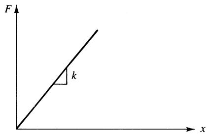Recall that a linear spring has force related to deformation by $\boldsymbol { F } = k \boldsymbol { x }$ , where k is the spring constant and x is the deformation of the spring (Figure 2–18). The differential internal work (or strain energy) dU in the spring for a small change in length of the spring is the internal force multiplied by the change in displacement through which the force moves, given by $$ d U = F d x \tag {2.6.2} $$ Now we express F as $$ F = k x \tag {2.6.3} $$ Using Eq. (2.6.3) in Eq. (2.6.2), we find that the differential strain energy becomes $$ d U = k x d x \tag {2.6.4} $$ 

text_image

F k x


text_image

k F x

Figure 2–18 Force/deformation curve for linear spring The total strain energy is then given by $$ U = \int_ {0} ^ {x} k x d x \tag {2.6.5} $$ Upon explicit integration of Eq. (2.6.5), we obtain $$ U = \frac {1}{2} k x ^ {2} \tag {2.6.6} $$ Using Eq. (2.6.3) in Eq. (2.6.6), we have $$ U = \frac {1}{2} (k x) x = \frac {1}{2} F x \tag {2.6.7} $$ Equation (2.6.7) indicates that the strain energy is the area under the force/deformation curve. The potential energy of the external force, being opposite in sign from the external work expression because the potential energy of the external force is lost when the work is done by the external force, is given by $$ \Omega = - F x \tag {2.6.8} $$ Therefore, substituting Eqs. 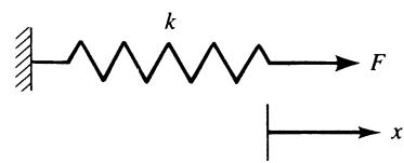(2.6.6) and (2.6.8) into (2.6.1), yields the total potential energy as $$ \pi_ {p} = \frac {1}{2} k x ^ {2} - F x \tag {2.6.9} $$ The concept of a stationary value of a function G (used in the definition of the principle of minimum potential energy) is shown in Figure 2–19. Here G is expressed as a function of the variable x. The stationary value can be a maximum, a minimum, or a neutral point of GðxÞ. To find a value of x yielding a stationary value of GðxÞ, we use differential calculus to differentiate G with respect to x and set the expression equal to zero, as follows: $$ \frac {d G}{d x} = 0 \tag {2.6.10} $$ An analogous process will subsequently be used to replace G with $\pi _ { p }$ and x with discrete values (nodal displacements) $d _ { i } .$ With an understanding of variational calculus (see Reference [8]), we could use the first variation of $\pi _ { p }$ (denoted by $\delta \pi _ { p } .$ , where $\delta$ denotes arbitrary change or variation) to minimize $\pi _ { p }$ . However, we will avoid the details of variational calculus and show that we can really use the familiar differential calculus to perform the minimization of $\pi _ { p }$ . To apply the principle of minimum 

line

| x | G | | ---- | ----- | | Minimum | Low | | Neutral | Peak | | Maximum | High |

Figure 2–19 Stationary values of a function 

text_image

Admissible displacement function, û + δû δû û₁ û₂ Actual displacement function, û 1 L 2 x̂ (a)


text_image

Inadmissible slope discontinuity û₁ û₂ Inadmissible—does not satisfy right end boundary condition 1 L 2 x̂ (b)

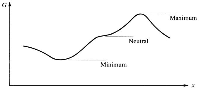
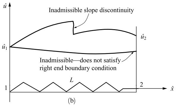
Figure 2–20 (a) Actual and admissible displacement functions and (b) inadmissible displacement functions potential energy—that is, to minimize $\pi _ { p } - \mathrm { w e }$ take the variation of $\pi _ { p }$ , which is a function of nodal displacements $d _ { i }$ defined in general as $$ \delta \pi_ {p} = \frac {\partial \pi_ {p}}{\partial d _ {1}} \delta d _ {1} + \frac {\partial \pi_ {p}}{\partial d _ {2}} \delta d _ {2} + \dots + \frac {\partial \pi_ {p}}{\partial d _ {n}} \delta d _ {n} \tag {2.6.11} $$ The principle states that equilibrium exists when the $d _ { i }$ define a structure state such that $\delta \pi _ { p } = 0$ (change in potential energy ¼ 0) for arbitrary admissible variations in displacement $\delta d _ { i }$ from the equilibrium state. An admissible variation is one in which the displacement field still satisfies the boundary conditions and interelement continuity. Figure 2–20(a) shows the hypothetical actual axial displacement and an admissible one for a spring with specified boundary displacements $\hat { u } _ { 1 }$ and $\hat { u } _ { 2 }$ . Figure 2–20(b) shows inadmissible functions due to slope discontinuity between endpoints 1 and 2 and due to failure to satisfy the right end boundary condition of $\hat { u } ( L ) = \hat { u } _ { 2 }$ . Here $\delta \hat { u }$ represents the variation in $\hat { u } .$ In the general finite element formulation, du^ would be replaced by $\delta d _ { i }$ . This implies that any of the $\delta d _ { i }$ might be nonzero. Hence, to satisfy $\delta \pi _ { p } = 0$ , all coefficients associated with the $\delta d _ { i }$ must be zero independently. Thus, $$ \frac {\partial \pi_ {p}}{\partial d _ {i}} = 0 \quad (i = 1, 2, 3, \dots , n) \quad \text { or } \quad \frac {\partial \pi_ {p}}{\partial \{d \}} = 0 \tag {2.6.12} $$ where n equations must be solved for the n values of $d _ { i }$ that define the static equilibrium state of the structure. Equation (2.6.12) shows that for our purposes throughout this text, we can interpret the variation of $\pi _ { p }$ as a compact notation equivalent to differentiation of $\pi _ { p }$ with respect to the unknown nodal displacements for which $\pi _ { p }$ is expressed. For linear-elastic materials in equilibrium, the fact that $\pi _ { p }$ is a minimum is shown, for instance, in Reference [4]. Before discussing the formulation of the spring element equations, we now illustrate the concept of the principle of minimum potential energy by analyzing a single-degree-of-freedom spring subjected to an applied force, as given in Example 2.4. In this example, we will show that the equilibrium position of the spring corresponds to the minimum potential energy. 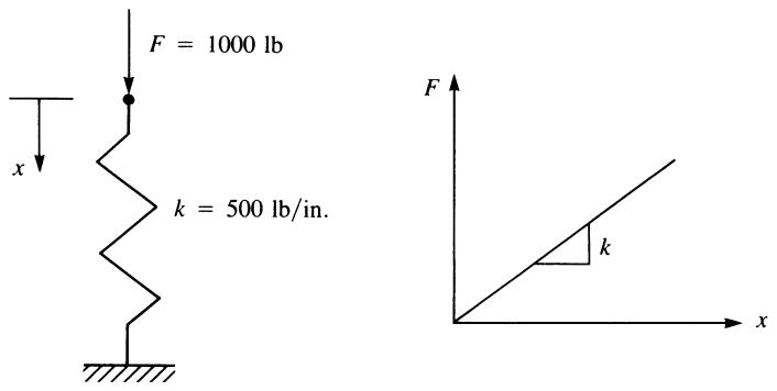# Example 2.4 For the linear-elastic spring subjected to a force of 1000 lb shown in Figure 2–21, evaluate the potential energy for various displacement values and show that the minimum potential energy also corresponds to the equilibrium position of the spring. 

text_image

F = 1000 lb k = 500 lb/in. F k x

Figure 2–21 Spring subjected to force; load/displacement curve We evaluate the total potential energy as $$ \pi_ {p} = U + \Omega $$ where $U = \textstyle { \frac { 1 } { 2 } } ( k x ) x \qquad { \mathrm { a n d } } \qquad \Omega = - F x$ We now illustrate the minimization of $\pi _ { p }$ through standard mathematics. Taking the variation of $\pi _ { p }$ with respect to x, or, equivalently, taking the derivative of $\pi _ { p }$ with respect to x (as $\pi _ { p }$ is a function of only one displacement x), as in Eqs. (2.6.11) and (2.6.12), we have $$ \delta \pi_ {p} = \frac {\partial \pi_ {p}}{\partial x} \delta x = 0 $$ or, because $\delta x$ is arbitrary and might not be zero, $$ \frac {\partial \pi_ {p}}{\partial x} = 0 $$ Using our previous expression for $\pi _ { p } .$ , we obtain $$ \frac {\partial \pi_ {p}}{\partial x} = 5 0 0 x - 1 0 0 0 = 0 $$ or x ¼ 2:00 in: This value for x is then back-substituted into $\pi _ { p }$ to yield $$ \pi_ {p} = 2 5 0 (2) ^ {2} - 1 0 0 0 (2) = - 1 0 0 0 \mathrm{lb-in}. $$ which corresponds to the minimum potential energy obtained in Table 2–1 by the following searching technique. Here $\begin{array} { r } { \bar { U } = \frac { 1 } { 2 } ( k x ) x } \end{array}$ is the strain energy or the area under the load/displacement curve shown in Figure 2–21, and $\Omega = - F x$ is the potential energy of load F. 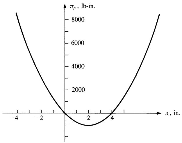For the given values of F and $k ,$ we then have $$ \pi_ {p} = \frac {1}{2} (5 0 0) x ^ {2} - 1 0 0 0 x = 2 5 0 x ^ {2} - 1 0 0 0 x $$ We now search for the minimum value of $\pi _ { p }$ for various values of spring deformation x. The results are shown in Table 2–1. A plot of $\pi _ { p }$ versus x is shown in Figure 2–22, where we observe that $\pi _ { p }$ has a minimum value at $x = 2 . 0 0$ in. This deformed position also corresponds to the equilibrium position because $( \hat { \sigma } \pi _ { p } / \hat { \sigma } x ) = 5 0 0 ( 2 ) - 1 0 0 0 = 0$ . 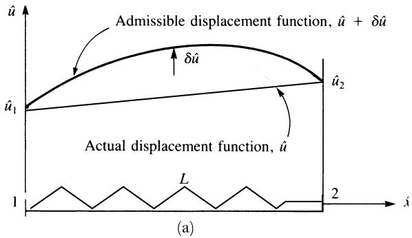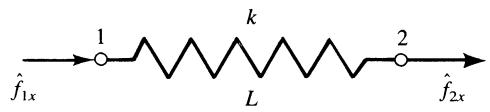We now derive the spring element equations and stiffness matrix using the principle of minimum potential energy. Consider the linear spring subjected to nodal forces shown in Figure 2–23. Using Eq. (2.6.9) reveals that the total potential energy is $$ \pi_ {p} = \frac {1}{2} k (\hat {d} _ {2 x} - \hat {d} _ {1 x}) ^ {2} - \hat {f} _ {1 x} \hat {d} _ {1 x} - \hat {f} _ {2 x} \hat {d} _ {2 x} \tag {2.6.13} $$ where $\hat { d } _ { 2 x } - \hat { d } _ { 1 x }$ is the deformation of the spring in Eq. (2.6.9). The first term on the right in Eq. (2.6.13) is the strain energy in the spring. Simplifying Eq. (2.6.13), we obtain $$ \pi_ {p} = \frac {1}{2} k \left(\hat {d} _ {2 x} ^ {2} - 2 \hat {d} _ {2 x} \hat {d} _ {1 x} + \hat {d} _ {1 x} ^ {2}\right) - \hat {f} _ {1 x} \hat {d} _ {1 x} - \hat {f} _ {2 x} \hat {d} _ {2 x} \tag {2.6.14} $$ Table 2–1 Total potential energy for various spring deformations

Deformation x, in.	Total Potential Energy πp, lb-in.
-4.00	8000
-3.00	5250
-2.00	3000
-1.00	1250
0.00	0
1.00	-750
2.00	-1000
3.00	-750
4.00	0
5.00	1250


line

| x, in. | πρ, lb-in. | |---|---| | -4 | 8000 | | -2 | 4000 | | 0 | 0 | | 2 | -4000 | | 4 | 0 | | 6 | 4000 | | 8 | 8000 |

Figure 2–22 Variation of potential energy with spring deformation 

text_image

f̂₁ₓ → 1 → k → 2 → f̂₂ₓ L

Figure 2–23 Linear spring subjected to nodal forces The minimization of $\pi _ { p }$ with respect to each nodal displacement requires taking partial derivatives of $\pi _ { p }$ with respect to each nodal displacement such that $$ \frac {\partial \pi_ {p}}{\partial \hat {d} _ {1 x}} = \frac {1}{2} k \left(- 2 \hat {d} _ {2 x} + 2 \hat {d} _ {1 x}\right) - \hat {f} _ {1 x} = 0 \tag {2.6.15} $$ $$ \frac {\partial \pi_ {p}}{\partial \hat {d} _ {2 x}} = \frac {1}{2} k (2 \hat {d} _ {2 x} - 2 \hat {d} _ {1 x}) - \hat {f} _ {2 x} = 0 $$ Simplifying Eqs. (2.6.15), we have $$ k \left(- \hat {d} _ {2 x} + \hat {d} _ {1 x}\right) = \hat {f} _ {1 x} \tag {2.6.16} $$ $$ k (\hat {d} _ {2 x} - \hat {d} _ {1 x}) = \hat {f} _ {2 x} $$ In matrix form, we express Eq. (2.6.16) as $$ \left[ \begin{array}{c c} k & - k \\ - k & k \end{array} \right] \left\{ \begin{array}{l} \hat {d} _ {1 x} \\ \hat {d} _ {2 x} \end{array} \right\} = \left\{ \begin{array}{l} \hat {f} _ {1 x} \\ \hat {f} _ {2 x} \end{array} \right\} \tag {2.6.17} $$ Because $\{ \hat { f } \} = \hat { \boldsymbol { k } } ] \{ \hat { d } \}$ , we have the stiffness matrix for the spring element obtained from Eq. (2.6.17): $$ [ \hat {k} ] = \left[ \begin{array}{c c} k & - k \\ - k & k \end{array} \right] \tag {2.6.18} $$ As expected, Eq. (2.6.18) is identical to the stiffness matrix obtained in Section 2.2, Eq. (2.2.18). We considered the equilibrium of a single spring element by minimizing the total potential energy with respect to the nodal displacements (see Example 2.4). We also developed the finite element spring element equations by minimizing the total potential energy with respect to the nodal displacements. We now show that the total potential energy of an entire structure (here an assemblage of spring elements) can be minimized with respect to each nodal degree of freedom and that this minimization results in the same finite element equations used for the solution as those obtained by the direct stiffness method. 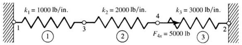# Example 2.5 Obtain the total potential energy of the spring assemblage (Figure 2–24) for Example 2.1 and find its minimum value. The procedure of assembling element equations can then be seen to be obtained from the minimization of the total potential energy. 

text_image

k₁ = 1000 lb/in. k₂ = 2000 lb/in. k₃ = 3000 lb/in. F₄ₓ = 5000 lb ① ② ③

Using Eq. (2.6.10) for each element of the spring assemblage, we find that the total potential energy is given by $$ \begin{array}{l} \pi_ {p} = \sum_ {e = 1} ^ {3} \pi_ {p} ^ {(e)} = \frac {1}{2} k _ {1} \left(d _ {3 x} - d _ {1 x}\right) ^ {2} - f _ {1 x} ^ {(1)} d _ {1 x} - f _ {3 x} ^ {(1)} d _ {3 x} \\ + \frac {1}{2} k _ {2} (d _ {4 x} - d _ {3 x}) ^ {2} - f _ {3 x} ^ {(2)} d _ {3 x} - f _ {4 x} ^ {(2)} d _ {4 x} \tag {2.6.19} \\ + \frac {1}{2} k _ {3} (d _ {2 x} - d _ {4 x}) ^ {2} - f _ {4 x} ^ {(3)} d _ {4 x} - f _ {2 x} ^ {(3)} d _ {2 x} \\ \end{array} $$ Upon minimizing $\pi _ { p }$ with respect to each nodal displacement, we obtain $$ \begin{array}{l} \frac {\partial \pi_ {p}}{\partial d _ {1 x}} = - k _ {1} d _ {3 x} + k _ {1} d _ {1 x} - f _ {1 x} ^ {(1)} = 0 \\ \frac {\partial \pi_ {p}}{\partial d _ {2 x}} = k _ {3} d _ {2 x} - k _ {3} d _ {4 x} - f _ {2 x} ^ {(3)} = 0 \tag {2.6.20} \\ \end{array} $$ $$ \frac {\partial \pi_ {p}}{\partial d _ {3 x}} = k _ {1} d _ {3 x} - k _ {1} d _ {1 x} - k _ {2} d _ {4 x} + k _ {2} d _ {3 x} - f _ {3 x} ^ {(1)} - f _ {3 x} ^ {(2)} = 0 $$ $$ \frac {\partial \pi_ {p}}{\partial d _ {4 x}} = k _ {2} d _ {4 x} - k _ {2} d _ {3 x} - k _ {3} d _ {2 x} + k _ {3} d _ {4 x} - f _ {4 x} ^ {(2)} - f _ {4 x} ^ {(3)} = 0 $$ In matrix form, Eqs. (2.6.20) become $$ \left[ \begin{array}{c c c c} k _ {1} & 0 & - k _ {1} & 0 \\ 0 & k _ {3} & 0 & - k _ {3} \\ - k _ {1} & 0 & k _ {1} + k _ {2} & - k _ {2} \\ 0 & - k _ {3} & - k _ {2} & k _ {2} + k _ {3} \end{array} \right] \left\{ \begin{array}{l} d _ {1 x} \\ d _ {2 x} \\ d _ {3 x} \\ d _ {4 x} \end{array} \right\} = \left\{ \begin{array}{c} f _ {1 x} ^ {(1)} \\ f _ {2 x} ^ {(3)} \\ f _ {3 x} ^ {(1)} + f _ {3 x} ^ {(2)} \\ f _ {4 x} ^ {(2)} + f _ {4 x} ^ {(3)} \end{array} \right\} \tag {2.6.21} $$ Using nodal force equilibrium similar to Eqs. (2.3.4)–(2.3.6), we have $$ f _ {1 x} ^ {(1)} = F _ {1 x} $$ $$ f _ {2 x} ^ {(3)} = F _ {2 x} \tag {2.6.22} $$ $$ f _ {3 x} ^ {(1)} + f _ {3 x} ^ {(2)} = F _ {3 x} $$ $$ f _ {4 x} ^ {(2)} + f _ {4 x} ^ {(3)} = F _ {4 x} $$ Using Eqs. (2.6.22) in (2.6.21) and substituting numerical values for $k _ { 1 } , k _ { 2 }$ , and $k _ { 3 ; }$ , we obtain $$ \left[ \begin{array}{c c c c} 1 0 0 0 & 0 & - 1 0 0 0 & 0 \\ 0 & 3 0 0 0 & 0 & - 3 0 0 0 \\ - 1 0 0 0 & 0 & 3 0 0 0 & - 2 0 0 0 \\ 0 & - 3 0 0 0 & - 2 0 0 0 & 5 0 0 0 \end{array} \right] \left\{ \begin{array}{l} d _ {1 x} \\ d _ {2 x} \\ d _ {3 x} \\ d _ {4 x} \end{array} \right\} = \left\{ \begin{array}{l} F _ {1 x} \\ F _ {2 x} \\ F _ {3 x} \\ F _ {4 x} \end{array} \right\} \tag {2.6.23} $$ Equation (2.6.23) is identical to Eq. (2.5.18), which was obtained through the direct stiffness method. The assembled Eqs. (2.6.23) are then seen to be obtained from the minimization of the total potential energy. When we apply the boundary conditions and substitute $F _ { 3 x } = 0$ and $F _ { 4 x } = 5 0 0 0$ lb into Eq. (2.6.23), the solution is identical to that of Example 2.1. 9 # References [1] Turner, M. J., Clough, R. W., Martin, H. C., and Topp, L. J., ‘‘Stiffness and Deflection Analysis of Complex Structures,’’ Journal of the Aeronautical Sciences, Vol. 23, No. 9, pp. 805–824, Sept. 1956. [2] Martin, H. C., Introduction to Matrix Methods of Structural Analysis, McGraw-Hill, New York, 1966. [3] Hsieh, Y. Y., Elementary Theory of Structures, 2nd ed., Prentice-Hall, Englewood Cliffs, NJ, 1982. [4] Oden, J. T., and Ripperger, E. A., Mechanics of Elastic Structures, 2nd ed., McGraw-Hill, New York, 1981. [5] Finlayson, B. A., The Method of Weighted Residuals and Variational Principles, Academic Press, New York, 1972. [6] Zienkiewicz, O. C., The Finite Element Method, 3rd ed., McGraw-Hill, London, 1977. [7] Cook, R. D., Malkus, D. S., Plesha, M. E., and Witt, R. J. Concepts and Applications of Finite Element Analysis, 4th ed., Wiley, New York, 2002. [8] Forray, M. J., Variational Calculus in Science and Engineering, McGraw-Hill, New York, 1968. 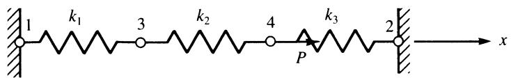# d Problems 2.1 a. Obtain the global stiffness matrix K of the assemblage shown in Figure P2–1 by superimposing the stiffness matrices of the individual springs. Here $k _ { 1 } , k _ { 2 }$ , and $k _ { 3 }$ are the stiffnesses of the springs as shown. b. If nodes 1 and 2 are fixed and a force P acts on node 4 in the positive x direction, find an expression for the displacements of nodes 3 and 4. c. Determine the reaction forces at nodes 1 and 2. (Hint: Do this problem by writing the nodal equilibrium equations and then making use of the force/displacement relationships for each element as done in the first part of Section 2.4. Then solve the problem by the direct stiffness method.) 

text_image

1 k₁ 3 k₂ 4 k₃ P 2 x

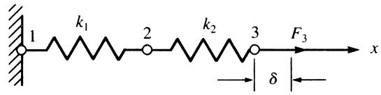
Figure P2–1 2.2 For the spring assemblage shown in Figure P2–2, determine the displacement at node 2 and the forces in each spring element. Also determine the force $F _ { 3 }$ . Given: Node 3 displaces an amount $\delta = 1$ in. in the positive x direction because of the force $F _ { 3 }$ and $k _ { 1 } = k _ { 2 } = 5 0 0$ lb/in. 

text_image

1 k₁ 2 k₂ 3 F₃ x δ

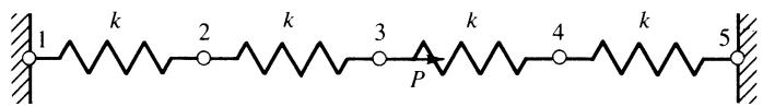
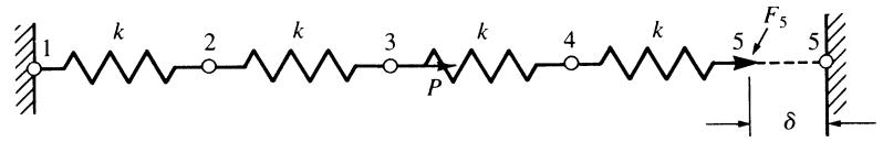
Figure P2–2 2.3 a. For the spring assemblage shown in Figure P2–3, obtain the global stiffness matrix by direct superposition. b. If nodes 1 and 5 are fixed and a force P is applied at node 3, determine the nodal displacements. c. Determine the reactions at the fixed nodes 1 and 5. 

text_image

1 k 2 k 3 k 4 k 5 P

Figure P2–3 2.4 Solve Problem 2.3 with P ¼ 0 (no force applied at node 3) and with node 5 given a fixed, known displacement of d as shown in Figure P2–4. 

text_image

1 k 2 k 3 k 4 k 5 F5 5 P δ

Figure P2–4 2.5 For the spring assemblage shown in Figure P2–5, obtain the global stiffness matrix by the direct stiffness method. Let $k ^ { ( 1 ) } = 1 \mathrm { { k i p } / \mathrm { { i n } . , } } k ^ { ( 2 ) } = 2 \mathrm { { k i p } / \mathrm { { i n } . , } } k ^ { ( 3 ) } = 3 \mathrm { { k i p } / \mathrm { { i n } . } }$ ; $k ^ { ( 4 ) } = 4$ kip/in., and $k ^ { ( 5 ) } = 5$ kip/in. 

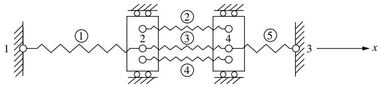
text_image

1 ① 2 ② 3 4 ③ ④ ⑤ 3 x

Figure P 2–5 2.6 For the spring assemblage in Figure P2–5, apply a concentrated force of 2 kips at node 2 in the positive x direction and determine the displacements at nodes 2 and 4. 2.7 Instead of assuming a tension element as in Figure P2–3, now assume a compression element. That is, apply compressive forces to the spring element and derive the stiffness matrix. 2.8–2.16 For the spring assemblages shown in Figures P2–8—P2–16, determine the nodal displacements, the forces in each element, and the reactions. Use the direct stiffness method for all problems. 

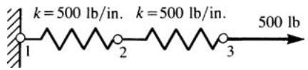
text_image

k = 500 lb/in. k = 500 lb/in. 1 2 3 500 lb

Figure P 2–8 

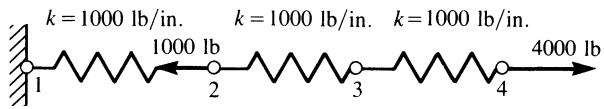
text_image

k = 1000 lb/in. 1000 lb k = 1000 lb/in. k = 1000 lb/in. 2 3 4 4000 lb

Figure P2–9 

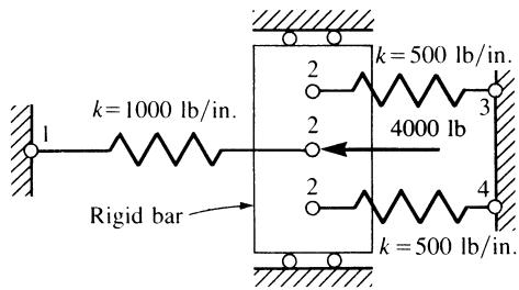
text_image

k=1000 lb/in. 2 k=500 lb/in. 4000 lb 1 2 2 4 k=500 lb/in. Rigid bar

Figure P2–10