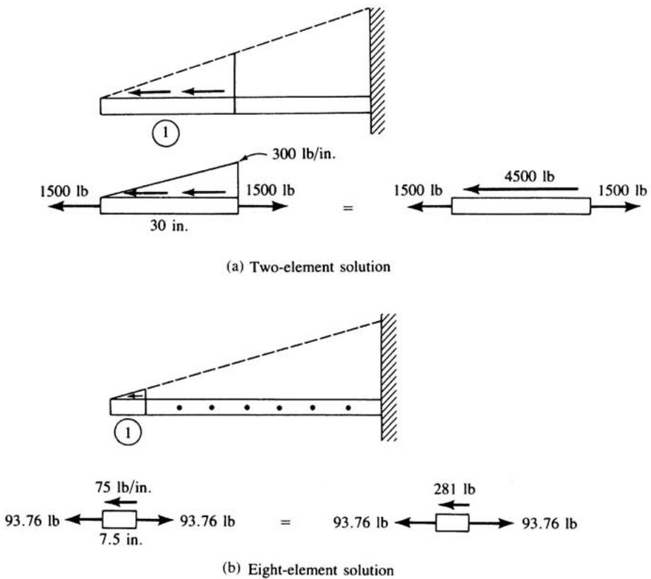
Figure 3–34 Free-body diagram of element 1 in both two- and eight-element models, showing that equilibrium is not satisfied 

line

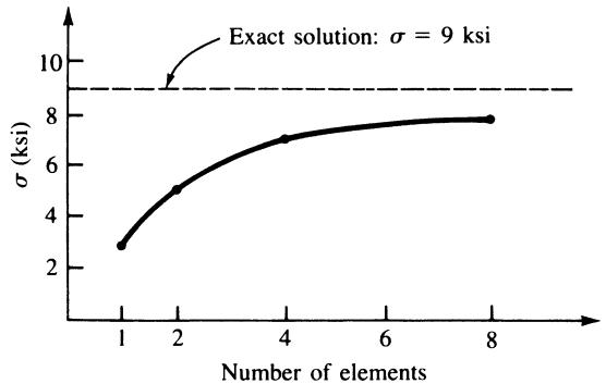
| Number of elements | σ (ksi) | | ------------------ | ------- | | 1 | 3 | | 2 | 5 | | 4 | 7 | | 8 | 8 |

Figure 3–35 Axial stress at fixed end as number of elements increases However, if we formulate the problem in a customary general way, as described in detail in Chapter 4 for beams subjected to distributed loading, we can obtain the exact stress distribution with any of the models used. That is, letting $\underline { { \hat { f } } } = \underline { { \hat { k } } } \underline { { \hat { d } } } - \underline { { \hat { f } } } _ { 0 } ,$ where $\underline { { \hat { f } } } _ { 0 }$ is the initial nodal replacement force system of the distributed load on each element, we subtract the initial replacement force system from the $\underline { { \hat { k } } } \underline { { \hat { d } } }$ result. This yields the nodal forces in each element. For example, considering element 1 of the two-element model, we have [see also Eqs. (3.10.33) and (3.10.41)] $$ \underline {{f}} _ {0} = \left\{ \begin{array}{l} - 1 5 0 0 \mathrm{lb} \\ - 3 0 0 0 \mathrm{lb} \end{array} \right\} $$ Using $\underline { { \hat { f } } } = \underline { { \hat { k } } } \underline { { \hat { d } } } - \underline { { \hat { f } } } _ { 0 } ,$ we obtain $$ \begin{array}{l} \underline {{\hat {f}}} = \frac {2 (3 0 \times 1 0 ^ {6})}{(3 0 \text { in. })} \left[ \begin{array}{c c} 1 & - 1 \\ - 1 & 1 \end{array} \right] \left\{ \begin{array}{c} - 0. 0 0 6 \text { in. } \\ - 0. 0 0 5 2 5 \text { in. 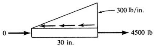} \end{array} \right\} - \left\{ \begin{array}{c} - 1 5 0 0 \text { lb } \\ - 3 0 0 0 \text { lb } \end{array} \right\} \\ = \left\{ \begin{array}{c} - 1 5 0 0 + 1 5 0 0 \\ 1 5 0 0 + 3 0 0 0 \end{array} \right\} = \left\{ \begin{array}{c} 0 \\ 4 5 0 0 \end{array} \right\} \\ \end{array} $$ as the actual nodal forces. Drawing a free-body diagram of element 1, we have 

text_image

0 → 30 in. 300 lb/in. 4500 lb

$$ \sum F _ {x} = 0: - \frac {1}{2} (3 0 0 \mathrm{lb/in.}) (3 0 \mathrm{in.}) + 4 5 0 0 \mathrm{lb} = 0 $$ For other kinds of elements (other than beams), this adjustment is ignored in practice. The adjustment is less important for plane and solid elements than for beams. Also, these adjustments are more difficult to formulate for an element of general shape. # d 3.12 Galerkin’s Residual Method and Its Use to Derive the One-Dimensional Bar Element Equations General Formulation We developed the bar finite element equations by the direct method in Section 3.1 and by the potential energy method (one of a number of variational methods) in Section 3.10. In fields other than structural/solid mechanics, it is quite probable that a variational principle, analogous to the principle of minimum potential energy, for instance, may not be known or even exist. In some flow problems in fluid mechanics and in mass transport problems (Chapter 13), we often have only the differential equation and boundary conditions available. However, the finite element method can still be applied. The methods of weighted residuals applied directly to the differential equation can be used to develop the finite element equations. In this section, we describe Galerkin’s residual method in general and then apply it to the bar element. This development provides the basis for later applications of Galerkin’s method to the beam element in Chapter 4 and to the nonstructural heat-transfer element (specifically, the one-dimensional combined conduction, convection, and mass transport element described in Chapter 13). Because of the mass transport phenomena, the variational formulation is not known (or certainly is difficult to obtain), so Galerkin’s method is necessarily applied to develop the finite element equations. There are a number of other residual methods. Among them are collocation, least squares, and subdomain as described in Section 3.13. (For more on these methods, see Reference [5].) In weighted residual methods, a trial or approximate function is chosen to approximate the independent variable, such as a displacement or a temperature, in a problem defined by a differential equation. This trial function will not, in general, satisfy the governing differential equation. Thus substituting the trial function into the differential equation results in a residual over the whole region of the problem as follows: $$ \iint_ {V} R d V = \text { minimum } \tag {3.12.1} $$ In the residual method, we require that a weighted value of the residual be a minimum over the whole region. The weighting functions allow the weighted integral of residuals to go to zero. If we denote the weighting function by W , the general form of the weighted residual integral is $$ \iint_ {V} R W d V = 0 \tag {3.12.2} $$ Using Galerkin’s method, we choose the interpolation function, such as Eq. (3.1.3), in terms of $N _ { i }$ shape functions for the independent variable in the differential equation. In general, this substitution yields the residual $R \neq 0$ . By the Galerkin criterion, the shape functions $N _ { i }$ are chosen to play the role of the weighting functions $W ,$ . Thus for each $i ,$ we have $$ \iint_ {V} R N _ {i} d V = 0 \quad (i = 1, 2, \dots , n) \tag {3.12.3} $$ Equation (3.12.3) results in a total of n equations. Equation (3.12.3) applies to points within the region of a body without reference to boundary conditions such as specified applied loads or displacements. To obtain boundary conditions, we apply integration by parts to Eq. (3.12.3), which yields integrals applicable for the region and its boundary. # Bar Element Formulation We now illustrate Galerkin’s method to formulate the bar element stiffness equations. We begin with the basic differential equation, without distributed load, derived in Section 3.1 as $$ \frac {d}{d \hat {x}} \left(A E \frac {d \hat {u}}{d \hat {x}}\right) = 0 \tag {3.12.4} $$ where constants A and E are now assumed. The residual R is now defined to be Eq. (3.12.4). Applying Galerkin’s criterion [Eq. (3.12.3)] to Eq. (3.12.4), we have $$ \int_ {0} ^ {L} \frac {d}{d \hat {x}} \left(A E \frac {d \hat {u}}{d \hat {x}}\right) N _ {i} d \hat {x} = 0 \quad (i = 1, 2) \tag {3.12.5} $$ We now apply integration by parts to Eq. (3.12.5). Integration by parts is given in general by $$ \int u d v = u v - \int v d u \tag {3.12.6} $$ where u and v are simply variables in the general equation. Letting $$ u = N _ {i} \quad d u = \frac {d N _ {i}}{d \hat {x}} d \hat {x} $$ $$ d v = \frac {d}{d \hat {x}} \left(A E \frac {d \hat {u}}{d \hat {x}}\right) d \hat {x} \quad v = A E \frac {d \hat {u}}{d \hat {x}} \tag {3.12.7} $$ in Eq. (3.12.5) and integrating by parts according to Eq. (3.12.6), we find that Eq. (3.12.5) becomes $$ \left. \left(N _ {i} A E \frac {d \hat {u}}{d \hat {x}}\right) \right| _ {0} ^ {L} - \int_ {0} ^ {L} A E \frac {d \hat {u}}{d \hat {x}} \frac {d N _ {i}}{d \hat {x}} d \hat {x} = 0 \tag {3.12.8} $$ where the integration by parts introduces the boundary conditions. Recall that, because $\hat { u } = [ N ] \{ \hat { d } \}$ , we have $$ \frac {d \hat {u}}{d \hat {x}} = \frac {d N _ {1}}{d \hat {x}} \hat {d} _ {1 x} + \frac {d N _ {2}}{d \hat {x}} \hat {d} _ {2 x} \tag {3.12.9} $$ or, when Eqs. (3.1.4) are used for $N _ { 1 } = 1 - \hat { x } / L$ and $N _ { 2 } = \hat { x } / L$ , $$ \frac {d \hat {u}}{d \hat {x}} = \left[ - \frac {1}{L} \quad \frac {1}{L} \right] \left\{ \begin{array}{l} \hat {d} _ {1 x} \\ \hat {d} _ {2 x} \end{array} \right\} \tag {3.12.10} $$ Using Eq. (3.12.10) in Eq. (3.12.8), we then express Eq. (3.12.8) as $$ A E \int_ {0} ^ {L} \frac {d N _ {i}}{d \hat {x}} \left[ - \frac {1}{L} \quad \frac {1}{L} \right] d \hat {x} \left\{ \begin{array}{l} \hat {d} _ {1 x} \\ \hat {d} _ {2 x} \end{array} \right\} = \left(N _ {i} A E \frac {d \hat {u}}{d \hat {x}}\right) \bigg | _ {0} ^ {L} \quad (i = 1, 2) \tag {3.12.11} $$ Equation (3.12.11) is really two equations (one for $N _ { i } = N _ { 1 }$ and one for $N _ { i } = N _ { 2 } )$ . First, using the weighting function $N _ { i } = N _ { 1 }$ , we have $$ A E \int_ {0} ^ {L} \frac {d N _ {1}}{d \hat {x}} \left[ - \frac {1}{L} \quad \frac {1}{L} \right] d \hat {x} \left\{ \begin{array}{l} \hat {d} _ {1 x} \\ \hat {d} _ {2 x} \end{array} \right\} = \left(N _ {1} A E \frac {d \hat {u}}{d \hat {x}}\right) \bigg | _ {0} ^ {L} \tag {3.12.12} $$ Substituting for $d N _ { 1 } / d \hat { x } ,$ we obtain $$ A E \int_ {0} ^ {L} \left[ - \frac {1}{L} \right] \left[ - \frac {1}{L} \quad \frac {1}{L} \right] d \hat {x} \left\{ \begin{array}{l} \hat {d} _ {1 x} \\ \hat {d} _ {2 x} \end{array} \right\} = \hat {f} _ {1 x} \tag {3.12.13} $$ where $\hat { f } _ { 1 x } = A E ( d \hat { u } / d \hat { x } )$ because $N _ { 1 } = 1$ at $x = 0$ and $N _ { 1 } = 0 { \mathrm { ~ a t ~ } } x = L$ . Evaluating Eq. (3.12.13) yields $$ \frac {A E}{L} (\hat {d} _ {1 x} - \hat {d} _ {2 x}) = \hat {f} _ {1 x} \tag {3.12.14} $$ Similarly, using $N _ { i } = N _ { 2 }$ , we obtain $$ A E \int_ {0} ^ {L} \left[ \frac {1}{L} \right] \left[ - \frac {1}{L} \quad \frac {1}{L} \right] d \hat {x} \left\{ \begin{array}{l} \hat {d} _ {1 x} \\ \hat {d} _ {2 x} \end{array} \right\} = \left. \left(N _ {2} A E \frac {d \hat {u}}{d \hat {x}}\right) \right| _ {0} ^ {L} \tag {3.12.15} $$ Simplifying Eq. (3.12.15) yields $$ \frac {A E}{L} (\hat {d} _ {2 x} - \hat {d} _ {1 x}) = \hat {f} _ {2 x} \tag {3.12.16} $$ where $\hat { f } _ { 2 x } = A E ( d \hat { u } / d \hat { x } )$ because $N _ { 2 } = 1$ at $x = L$ and $N _ { 2 } = 0$ at $x = 0$ . Equations (3.12.14) and (3.12.16) are then seen to be the same as Eqs. (3.1.13) and (3.10.27) derived, respectively, by the direct and the variational method. 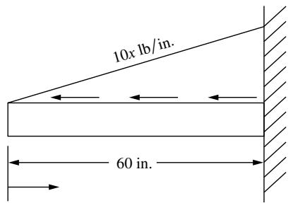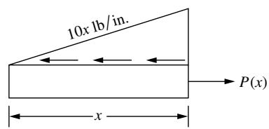# 3.13 Other Residual Methods and Their Application to a One-Dimensional Bar Problem As indicated in Section 3.12 when describing Galerkin’s residual method, weighted residual methods are based on assuming an approximate solution to the governing differential equation for the given problem. The assumed or trial solution is typically a displacement or a temperature function that must be made to satisfy the initial and boundary conditions of the problem. This trial solution will not, in general, satisfy the governing differential equation. Thus, substituting the trial function into the differential equation will result in some residuals or errors. Each residual method requires the error to vanish over some chosen intervals or at some chosen points. To demonstrate this concept, we will solve the problem of a rod subjected to a triangular load distribution as shown in Figure 3–29 (see Section 3.10) for which we also have an exact solution for the axial displacement given by Eq. (3.11.5) in Section 3.11. We will illustrate four common weighted residual methods: collocation, subdomain, least squares, and Galerkin’s method. It is important to note that the primary intent in this section is to introduce you to the general concepts of these other weighted residual methods through a simple 

text_image

10x lb/in. 60 in.

(a) 

text_image

10x lb/in. x P(x)

(b) Figure 3–36 (a) Rod subjected to triangular load distribution and (b) free-body diagram of section of rod example. You should note that we will assume a displacement solution that will in general yield an approximate solution (in our example the assumed displacement function yields an exact solution) over the whole domain of the problem (the rod previously solved in Section 13.10). As you have seen already for the spring and bar elements, we have assumed a linear function over each spring or bar element, and then combined the element solutions as was illustrated in Section 3.10 for the same rod solved in this section. It is common practice to use the simple linear function in each element of a finite element model, with an increasing number of elements used to model the rod yielding a closer and closer approximation to the actual displacement as seen in Figure 3–32. For clarity’s sake, Figure 3–36(a) shows the problem we are solving, along with a free-body diagram of a section of the rod with the internal axial force $P ( x )$ shown in Figure 3–36(b). The governing differential equation for the axial displacement, u, is given by $$ \left(A E \frac {d u}{d x}\right) - P (x) = 0 \tag {3.13.1} $$ where the internal axial force is $P ( x ) = 5 x ^ { 2 }$ . The boundary condition is $u ( x = L ) = 0$ The method of weighted residuals requires us to assume an approximation function for the displacement. This approximate solution must satisfy the boundary condition of the problem. Here we assume the following function: $$ u (x) = c _ {1} (x - L) + c _ {2} (x - L) ^ {2} + c _ {3} (x - L) ^ {3} \tag {3.13.2} $$ where $c _ { 1 } , \ : c _ { 2 }$ and $c _ { 3 }$ are unknown coefficients. Equation (3.13.2) also satisfies the boundary condition given by $u ( x = L ) = 0$ . Substituting Eq. (3.13.2) for u into the governing differential equation, Eq. (3.13.1), results in the following error function, $R \colon$ $$ A E [ c _ {1} + 2 c _ {2} (x - L) + 3 c _ {3} (x - L) ^ {2} ] - 5 x ^ {2} = R \tag {3.13.3} $$ We now illustrate how to solve the governing differential equation by the four weighted residual methods. # Collocation Method The collocation method requires that the error or residual function, R, be forced to zero at as many points as there are unknown coefficients. Equation (3.13.2) has three unknown coefficients. Therefore, we will make the error function equal zero at three points along the rod. We choose the error function to go to zero at $x = 0 , x = L / 3$ , and $x = 2 L / 3$ as follows: $$ R (c, x = 0) = 0 = A E \left[ c _ {1} + 2 c _ {2} (- L) + 3 c _ {3} (- L) ^ {2} \right] = 0 $$ $$ R (c, x = L / 3) = 0 = A E [ c _ {1} + 2 c _ {2} (- 2 L / 3) + 3 c _ {3} (- 2 L / 3) ^ {2} ] - 5 (L / 3) ^ {2} = 0 \tag {3.13.4} $$ $$ R (c, x = 2 L / 3) = 0 = A E \left[ c _ {1} + 2 c _ {2} (- L / 3) + 3 c _ {3} (- L / 3) ^ {2} \right] - 5 (2 L / 3) ^ {2} = 0 $$ The three linear equations, Eq. (3.13.4), can now be solved for the unknown coefficients, $c _ { 1 } , \ : c _ { 2 }$ and $c _ { 3 }$ . The result is $$ c _ {1} = 5 L ^ {2} / (A E) \quad c _ {2} = 5 L / (A E) \quad c _ {3} = 5 / (3 A E) \tag {3.13.5} $$ Substituting the numerical values, A ¼ 2, $E = 3 0 \times 1 0 ^ { 6 }$ , and $L = 6 0$ into Eq. (3.13.5), we obtain the $c { \mathrm { { s } } }$ as: $$ c _ {1} = 3 \times 1 0 ^ {- 4}, \quad c _ {2} = 5 \times 1 0 ^ {- 6}, \quad c _ {3} = 2. 7 7 8 \times 1 0 ^ {- 8} \tag {3.13.6} $$ Substituting the numerical values for the coefficients given in Eq. (3.13.6) into Eq. (3.13.2), we obtain the final expression for the axial displacement as $$ u (x) = 3 \times 1 0 ^ {- 4} (x - L) + 5 \times 1 0 ^ {- 6} (x - L) ^ {2} + 2. 7 7 8 \times 1 0 ^ {- 8} (x - L) ^ {3} \tag {3.13.7} $$ Because we have chosen a cubic displacement function, Eq. (3.13.2), and the exact solution, Eq. (3.11.6), is also cubic, the collocation method yields the identical solution as the exact solution. The plot of the solution is shown in Figure 3–32 on page 121. # Subdomain Method The subdomain method requires that the integral of the error or residual function over some selected subintervals be set to zero. The number of subintervals selected must equal the number of unknown coefficients. Because we have three unknown coefficients in the rod example, we must make the number of subintervals equal to three. We choose the subintervals from $0$ to $L / 3 { \mathrm { . } }$ , from $L / 3$ to $2 L / 3 { \mathrm { , } }$ and from $2 L / 3$ to L as follows: $$ \begin{array}{l} \int_ {0} ^ {L / 3} R d x = 0 = \int_ {0} ^ {L / 3} \left\{A E \left[ c _ {1} + 2 c _ {2} (x - L) + 3 c _ {3} (x - L) ^ {2} \right] - 5 x ^ {2} \right\} d x \\ \int_ {L / 3} ^ {2 L / 3} R d x = 0 = \int_ {L / 3} ^ {2 L / 3} \left\{A E \left[ c _ {1} + 2 c _ {2} (x - L) + 3 c _ {3} (x - L) ^ {2} \right] - 5 x ^ {2} \right\} d x \tag {3.13.8} \\ \int_ {2 L / 3} ^ {L} R d x = 0 = \int_ {2 L / 3} ^ {L} \left\{A E \left[ c _ {1} + 2 c _ {2} (x - L) + 3 c _ {3} (x - L) ^ {2} \right] - 5 x ^ {2} \right\} d x \\ \end{array} $$ where we have used Eq. (3.13.3) for R in Eqs. (3.13.8). Integration of Eqs. (3.13.8) results in three simultaneous linear equations that can be solved for the coefficients $c _ { 1 } , \ : c _ { 2 }$ and $c _ { 3 }$ . Using the numerical values for A, $E ,$ and L as previously done, the three coefficients are numerically identical to those given by Eq. (3.13.6). The resulting axial displacement is then identical to Eq. (3.13.7). # Least Squares Method The least squares method requires the integral over the length of the rod of the error function squared to be minimized with respect to each of the unknown coefficients in the assumed solution, based on the following: $$ \frac {\partial}{\partial c _ {i}} \left(\int_ {0} ^ {L} R ^ {2} d x\right) = 0 \quad i = 1, 2, \dots N (\text { for } N \text { unknown coefficients }) \tag {3.13.9} $$ or equivalently to $$ \int_ {0} ^ {L} R \frac {\partial R}{\partial c _ {i}} d x = 0 \tag {3.13.10} $$ Because we have three unknown coefficients in the approximate solution, we will perform the integration three times according to Eq. (3.13.10) with three resulting equations as follows: $$ \begin{array}{l} \int_ {0} ^ {L} \left\{A E \left[ c _ {1} + 2 c _ {2} (x - L) + 3 c _ {3} (x - L) ^ {2} \right] - 5 x ^ {2} \right\} A E d x = 0 \\ \int_ {0} ^ {L} \left\{A E \left[ c _ {1} + 2 c _ {2} (x - L) + 3 c _ {3} (x - L) ^ {2} \right] - 5 x ^ {2} \right\} A E 2 (x - L) d x = 0 \tag {3.13.11} \\ \int_ {0} ^ {L} \left\{A E \left[ c _ {1} + 2 c _ {2} (x - L) + 3 c _ {3} (x - L) ^ {2} \right] - 5 x ^ {2} \right\} A E 3 (x - L) ^ {2} d x = 0 \\ \end{array} $$ In the first, second, and third of Eqs. (3.13.11), respectively, we have used the following partial derivatives: $$ \frac {\partial R}{\partial c _ {1}} = A E, \quad \frac {\partial R}{\partial c _ {2}} = A E 2 (x - L), \quad \frac {\partial R}{\partial c _ {3}} = A E 3 (x - L) ^ {2} \tag {3.13.12} $$ Integration of Eqs. (3.13.11) yields three linear equations that are solved for the three coefficients. The numerical values of the coefficients again are identical to those of Eq. (3.13.6). Hence, the solution is identical to the exact solution. # Galerkin’s Method Galerkin’s method requires the error to be orthogonal1 to some weighting functions $W _ { i }$ as given previously by Eq. (3.12.2). For the rod example, this integral becomes $$ \int_ {0} ^ {L} R W _ {i} d x = 0 \quad I = 1, 2, \dots , N \tag {3.13.13} $$ The weighting functions are chosen to be a part of the approximate solution. Because we have three unknown constants in the approximate solution, we need to generate three equations. Recall that the assumed solution is the cubic given by Eq. (3.13.2); therefore, we select the weighting functions to be $$ W _ {1} = x - L \quad W _ {2} = (x - L) ^ {2} \quad W _ {3} = (x - L) ^ {3} \tag {3.13.14} $$ Using the weighting functions from Eq. (3.13.14) successively in Eq. (3.13.13), we generate the following three equations: $$ \begin{array}{l} \int_ {0} ^ {L} \left\{A E \left[ c _ {1} + 2 c _ {2} (x - L) + 3 c _ {3} (x - L) ^ {2} \right] - 5 x ^ {2} \right\} (x - L) d x = 0 \\ \int_ {0} ^ {L} \left\{A E \left[ c _ {1} + 2 c _ {2} (x - L) + 3 c _ {3} (x - L) ^ {2} \right] - 5 x ^ {2} \right\} (x - L) ^ {2} d x = 0 \tag {3.13.15} \\ \int_ {0} ^ {L} \left\{A E \left[ c _ {1} + 2 c _ {2} (x - L) + 3 c _ {3} (x - L) ^ {2} \right] - 5 x ^ {2} \right\} (x - L) ^ {3} d x = 0 \\ \end{array} $$ Integration of Eqs. (3.13.15) results in three linear equations that can be solved for the unknown coefficients. The numerical values are the same as those given by Eq. (3.13.6). Hence, the solution is identical to the exact solution. In conclusion, because we assumed the approximate solution in the form of a cubic in x and the exact solution is also a cubic in x, all residual methods have yielded the exact solution. The purpose of this section has still been met to illustrate the four common residual methods to obtain an approximate (or exact in this example) solution to a known differential equation. The exact solution is shown by Eq. (3.11.6) and in Figure 3–32 in Section 3.11. # References [1] Turner, M. J., Clough, R. W., Martin, H. C., and Topp, L. J., ‘‘Stiffness and Deflection Analysis of Complex Structures,’’ Journal of the Aeronautical Sciences, Vol. 23, No. 9, Sept. 1956, pp. 805–824. [2] Martin, H. C., ‘‘Plane Elasticity Problems and the Direct Stiffness Method,’’ The Trend in Engineering, Vol. 13, Jan. 1961, pp. 5–19. [3] Melosh, R. J., ‘‘Basis for Derivation of Matrices for the Direct Stiffness Method,’’ Journal of the American Institute of Aeronautics and Astronautics, Vol. 1, No. 7, July 1963, pp. 1631–1637. [4] Oden, J. T., and Ripperger, E. A., Mechanics of Elastic Structures, 2nd ed., McGraw-Hill, New York, 1981. [5] Finlayson, B. A., The Method of Weighted Residuals and Variational Principles, Academic Press, New York, 1972. [6] Zienkiewicz, O. C., The Finite Element Method, 3rd ed., McGraw-Hill, London, 1977. [7] Cook, R. D., Malkus, D. S., Plesha, M. E., and Witt, R. J., Concepts and Applications of Finite Element Analysis, 4th ed., Wiley, New York, 2002. [8] Forray, M. J., Variational Calculus in Science and Engineering, McGraw-Hill, New York, 1968. [9] Linear Stress and Dynamics Reference Division, Docutech On-Line Documentation, Algor Interactive Systems, Pittsburgh, PA. 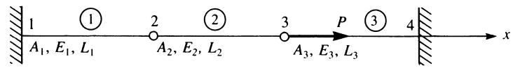# Problems 3.1 a. Compute the total stiffness matrix K of the assemblage shown in Figure P3–1 by superimposing the stiffness matrices of the individual bars. Note that K should be in terms of $A _ { 1 } , A _ { 2 } , A _ { 3 } , E _ { 1 } , E _ { 2 } , E _ { 3 } , L _ { 1 } , L _ { 2 }$ , and $L _ { 3 }$ . Here A; E, and L are generic symbols used for cross-sectional area, modulus of elasticity, and length, respectively. 

text_image

1 A₁, E₁, L₁ ① 2 A₂, E₂, L₂ ② 3 A₃, E₃, L₃ P ③ 4 x

Figure P3–1 b. Now let $A _ { 1 } = A _ { 2 } = A _ { 3 } = A , E _ { 1 } = E _ { 2 } = E _ { 3 } = E$ , and $L _ { 1 } = L _ { 2 } = L _ { 3 } = L$ . If nodes 1 and 4 are fixed and a force P acts at node 3 in the positive x direction, find expressions for the displacement of nodes 2 and 3 in terms of $A , E , L ,$ and P. c. Now let $A = 1 ~ \mathrm { i n } ^ { 2 }$ , $E = 1 0 \times 1 0 ^ { 6 }$ psi, L ¼ 10 in., and $P = 1 0 0 0 1 { \mathrm { b } } .$ . i. Determine the numerical values of the displacements of nodes 2 and 3. ii. Determine the numerical values of the reactions at nodes 1 and 4. iii. Determine the stresses in elements 1–3. 3.2–3.11 For the bar assemblages shown in Figures P3–2–P3–11, determine the nodal displacements, the forces in each element, and the reactions. Use the direct stiffness method for these problems.