text_image

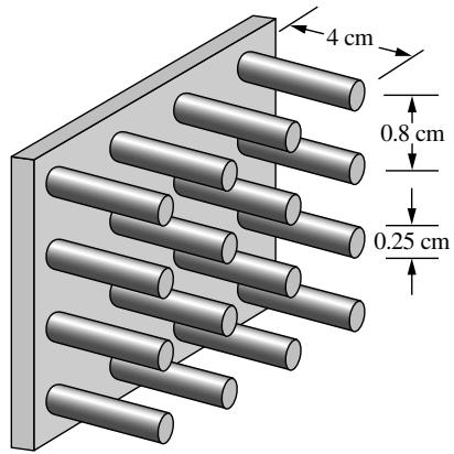
4 cm 0.8 cm 0.25 cm

Figure P13–15 

text_image

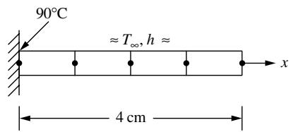
90°C ≈T∞, h ≈ x 4 cm

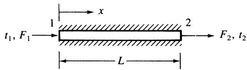
13.16 Use the direct method to derive the element equations for the one-dimensional steadystate conduction heat-transfer problem shown in Figure P13–16. The bar is insulated all around and has cross-sectional area A, length $L _ { \mathrm { { ; } } }$ and thermal conductivity $K _ { x x } .$ . Determine the relationship between nodal temperatures $t _ { 1 }$ and $t _ { 2 } \ ( ^ { \circ } \mathrm { F } )$ and the thermal inputs $F _ { 1 }$ and $F _ { 2 }$ (in Btu). Use Fourier’s law of heat conduction for this case. 

text_image

t₁, F₁ → 1 → x 2 → F₂, t₂ L →

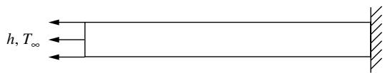
Figure P13–16 13.17 Express the stiffness matrix and the force matrix for convection from the left end of a bar, as shown in Figure P13–17. Let the cross-sectional area of the bar be $A ,$ the convection coefficient be h and the free stream temperature be $T _ { \infty }$ . 

text_image

h, T∞

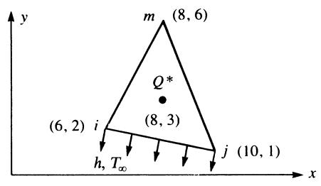
Figure P13–17 13.18 For the element shown in Figure P13–18, determine the $\underline { { k } }$ and $\underline { { f } }$ matrices. The conductivities are $K _ { x x } = K _ { y y } = 1 5 \ \mathrm { B t u } / ( \mathrm { h – f t – ^ { \circ } F } )$ and the convection coefficient is h ¼ 20 $\mathrm { B t u } / ( \mathrm { h - f t ^ { 2 } - ^ { \circ } F } )$ . Convection occurs across the $i \mathrm { - } j$ surface. The free-stream temperature is $T _ { \infty } = 7 0 ^ { \circ } \mathrm { F }$ . The coordinates are expressed in units of feet. Let the line source be Q ¼ 150 Btu/(h-ft) as located in the figure. Take the thickness of the element to be 1 ft. 

text_image

y m (8, 6) Q* (8, 3) (6, 2) i h, T∞ j (10, 1) x

Figure P13–18 

text_image

y m (0, 6) h Q* at (0, 0) (4, 0) x j (-2, -2) i

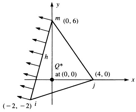
Figure P13–19 13.19 Calculate the $\underline { { k } }$ and $\underline { { f } }$ matrices for the element shown in Figure P13–19. The conductivities are $K _ { x x } = K _ { y y } = 1 5 \mathrm { \ W / ( m \cdot ^ { \circ } C ) }$ and the convection coefficient is $h =$ $2 0 \ \mathrm { W } / ( \mathrm { m } ^ { 2 } \cdot { } ^ { \circ } \mathrm { C } )$ . Convection occurs across the i-m surface. The free-stream temperature is $T _ { \infty } = 1 5 ^ { \circ } \mathrm { C }$ . The coordinates are shown expressed in units of meters. Let the line source be $Q ^ { * } = 1 0 0$ W/m as located in the figure. Take the thickness of the element to be 1 m. 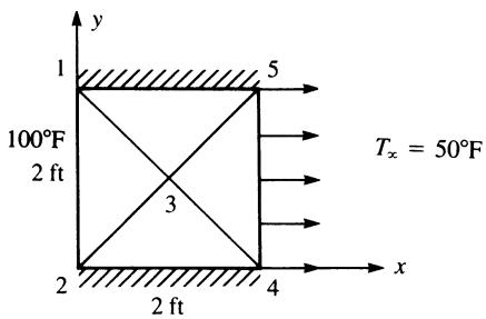13.20 For the square two-dimensional body shown in Figure P13–20, determine the temperature distribution. Let $K _ { x x } = K _ { y y } = 2 5 \mathrm { B t u } / ( \mathrm { h – f t – ^ { \circ } F } )$ and $h = 1 0 ~ \mathrm { B t u } / ( \mathrm { h } \mathrm { - f t } ^ { 2 } \mathrm { - } ^ { \circ } \mathrm { F } )$ . Convection occurs across side 4–5. The free-stream temperature is $T _ { \infty } = 5 0 ^ { \circ } \mathrm { F }$ . The temperatures at nodes 1 and 2 are $1 0 0 ^ { \circ } \mathrm { F }$ . The dimensions of the body are shown in the figure. Take the thickness of the body to be 1 ft. 

text_image

1 100°F 2 ft 3 2 ft 4 x 5 Tx = 50°F

Figure P13–20 

text_image

200°C 100°C 1 m t = 10 mm T∞ = 50°C

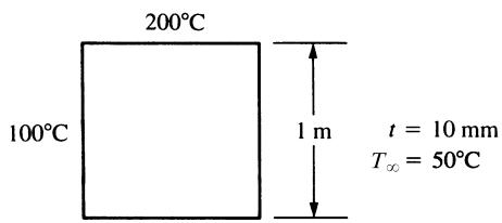
Figure P13–21 13.21 For the square plate shown in Figure P13–21, determine the temperature distribution. Let $K _ { x x } = K _ { y y } = 1 0 \mathrm { \ W / ( m \cdot ^ { \circ } C ) }$ and $h = 2 0 \ \mathrm { W } / ( \mathrm { m } ^ { 2 } \cdot { } ^ { \circ } \mathrm { C } )$ . The temperature along the left side is maintained at $1 0 0 ^ { \circ } \mathrm { C }$ and that along the top side is maintained at $2 0 0 ^ { \circ } \mathrm { C }$ . Use a computer program to calculate the temperature distribution in the following twodimensional bodies. 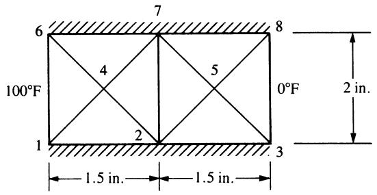13.22 For the body shown in Figure P13–22, determine the temperature distribution. Surface temperatures are shown in the figure. The body is insulated along the top and bottom edges, and $K _ { x x } = K _ { y y } = 1 . 0 \mathrm { B t u } / ( \mathrm { h – i n . ^ { \circ } F } )$ . No internal heat generation is present.  

text_image

6 7 8 100°F 4 5 0°F 2 in. 1 2 3 1.5 in. 1.5 in.

Figure P13–22 

text_image

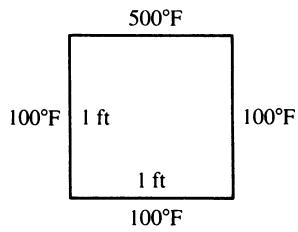
500°F 100°F 1 ft 100°F 1 ft 100°F

Figure P13–23 13.23 For the square two-dimensional body shown in Figure P13–23, determine the temperature distribution. Let $K _ { x x } = K _ { y y } = 1 0 \mathrm { B t u } / ( \mathrm { h – f t – ^ { \circ } F } )$ . The top surface is maintained at $5 0 0 ^ { \circ } \mathrm { F }$ and the other three sides are maintained at $\mathrm { i 0 0 ^ { \circ } F }$ . Also, plot the temperature contours on the body. 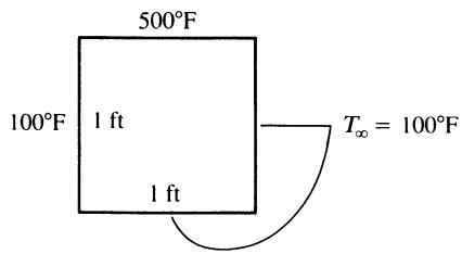13.24 For the square two-dimensional body shown in Figure P13–24, determine the temperature distribution. Let $K _ { x x } = K _ { y y } = 1 0 \mathrm { B t u } / ( \mathrm { h – f t – ^ { \circ } F } )$ and $h = 1 0 ~ \mathrm { B t u } / ( \mathrm { h } \mathrm { - f t } ^ { 2 } \mathrm { - } ^ { \circ } \mathrm { F } )$ . The top face is maintained at 500 F, the left face is maintained at $1 0 0 ^ { \circ } \mathrm { F }$ , and the other two faces are exposed to an environmental (free-stream) temperature of $1 0 0 ^ { \circ } \mathrm { F }$ . Also, plot the temperature contours on the body.   

text_image

500°F 100°F 1 ft 1 ft T∞ = 100°F

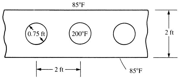
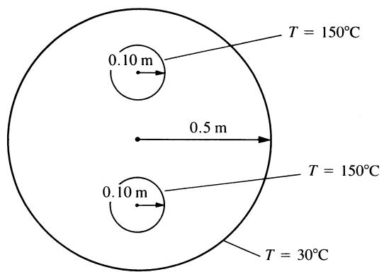
Figure P13–24 13.25 Hot water pipes are located on 2.0-ft centers in a concrete slab with $K _ { x x } = K _ { y y } = 0 . 8 0$ $\mathrm { B t u / ( h \mathrm { - } f t \mathrm { - } ^ { \circ } F ) }$ , as shown in Figure P13–25. If the outside surfaces of the concrete are at $8 5 ^ { \circ } \mathrm { F }$ and the water has an average temperature of $2 0 0 ^ { \circ } \mathrm { F }$ , determine the temperature distribution in the concrete slab. Plot the temperature contours through the concrete. Use symmetry in your finite element model. 

text_image

85°F 0.75 ft 200°F 2 ft 2 ft 85°F

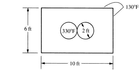
Figure P13–25 13.26 The cross section of a tall chimney shown in Figure P13–26 has an inside surface temperature of $3 3 0 ^ { \circ } \mathrm { F }$ and an exterior temperature of $1 3 0 ^ { \circ } \mathrm { F }$ . The thermal conductivity is $K = 0 . 5 ~ \mathrm { B t u } / ( \mathrm { h } \mathrm { - f t } { \mathrm { - } } ^ { \circ } \mathrm { F } )$ . Determine the temperature distribution within the chimney per unit length. 

text_image

6 ft 330°F 2 ft 10 ft 130°F

Figure P13–26 

text_image

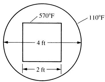
570°F 110°F 4 ft 2 ft

Figure P13–27 13.27 The square duct shown in Figure P13–27 carries hot gases such that its surface temperature is $5 7 0 ^ { \circ } \mathrm { F }$ . The duct is insulated by a layer of circular fiberglass that has a thermal conductivity of $K = 0 . 0 2 0 ~ \mathrm { B t u } / ( \mathrm { h } \mathrm { - f t } \cdot ^ { \circ } \mathrm { F } )$ . The outside surface temperature of the fiberglass is maintained at $1 1 0 ^ { \circ } \mathrm { F }$ . Determine the temperature distribution within the fiberglass. 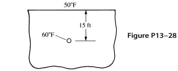13.28 The buried pipeline in Figure P13–28 transports oil with an average temperature of $6 0 ^ { \circ } \mathrm { F } .$ . The pipe is located 15 ft below the surface of the earth. The thermal conductivity of the earth is $0 . 6 \ \mathrm { B t u } / ( \mathrm { h } \mathrm { - f } \mathrm { t } \mathrm { - } ^ { \circ } \mathrm { F } )$ . The surface of the earth is $5 0 ^ { \circ } \mathrm { F }$ . Determine the temperature distribution in the earth. 

text_image

50°F 60°F 15 ft Figure P13-28

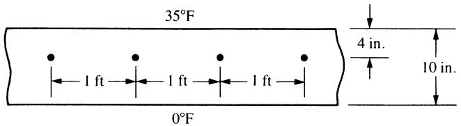
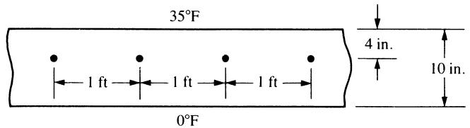
13.29 A 10-in.-thick concrete bridge deck is embedded with heating cables, as shown in A 10-in.-thick concrete bridge deck is embedded with heating cables,as shown in Figure P13–29. If the lower surface is at Figure P13-29. If the lower surface is at $0 ^ { \circ } \mathrm { F }$ , the rate of heat generation (assumed to , the rate of heat generation (assumed to be the same in each cable) is 100 Btu/(h-in.) and the top surface of the concrete is at be the same in each cable) is 1Oo Btu/(h-in.)and the top surface of the concrete is at $3 5 ^ { \circ } \mathrm { F }$ . The thermal conductivity of the concrete is 0.500 Btu/(h-ft-F). What is the . The thermal conductivity of the concrete is 0.50o Btu/(h-ft-°F). What is the temperature distribution in the slab? Use symmetry in your model. temperature distribution in the slab? Use symmetry in your model. 

text_image

35°F 1 ft 1 ft 1 ft 0°F 4 in. 10 in.

Figure P13–29 

text_image

T = 150°C 0.10 m 0.5 m T = 150°C 0.10 m T = 30°C

Figure P13–30 Figure P13-30 

text_image

100°C 0°C— 1 m 1 m T∞ = 0°C

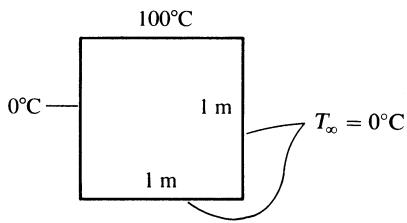
Figure P13–31 Figure P13-31 13.31 For the square two-dimensional body shown in Figure P13–31, determine the tem- 13.31 For the square two-dimensional body shown in Figure Pl3-31, determine the temperature distribution. Let perature distribution. Let $K _ { x x } = K _ { \nu \nu } = 1 0 ~ \mathrm { W / ( m \cdot ^ { \circ } C ) }$ and and $h = 1 0 \mathrm { ~ W } / ( \mathrm { m } ^ { 2 } \cdot \mathrm { ^ { \circ } C } )$ . The . The top face is maintained at top face is maintained at $1 0 0 ^ { \circ } \mathrm { C } ,$ , the left face is maintained at ,the left face is maintained at $0 ^ { \circ } \mathrm { C } .$ , and the other two ,and the other two faces are exposed to a free-stream temperature of faces are exposed to a free-stream temperature of $0 ^ { \circ } \mathbf { C }$ . Also, plot the temperature . Also,plot the temperature contours on the body. contours on the body. 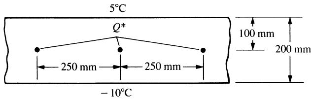13.32 A 200-mm-thick concrete bridge deck is embedded with heating cables as shown 13.32 A 200-mm-thick concrete bridge deck is embedded with heating cables as shown in Figure P13–32. If the lower surface is at in Figure Pl3-32. If the lower surface is at $- 1 0 ^ { \circ } \mathrm { C }$ and the upper surface is at and the upper surface is at $5 ^ { \circ } \mathrm { C } ,$ what is the temperature distribution in the slab? The heating cables are line sources what is the temperature distribution in the slab? The heating cables are line sources generating heat of generating heat of $Q ^ { * } = 5 0 ~ \mathrm { W / m }$ . The thermal conductivity of the concrete is 1.2 W/ . The thermal conductivity of the concrete is 1.2 W/ $( \mathbf { m } \cdot \mathbf { \vec { C } } )$ . Use symmetry in your model. . Use symmetry in your model.          

text_image

35°F 1 ft 1 ft 1 ft 0°F 4 in. 10 in.

13.30 For the circular body with holes shown in Figure P13–30, determine the temperature 13.30 For the circular body with holes shown in Figure P13-30, determine the temperature 13.30 For the circular body with holes shown in Figure P13-30, determine the temperature 13.30 For the circular body with holes shown in Figure P13-30, determine the temperature distribution. The inside surfaces of the holes have temperatures of distribution. The inside surfaces of the holes have temperatures of distribution. The inside surfaces of the holes have temperatures of distribution. The inside surfaces of the holes have temperatures of $1 5 0 ^ { \circ } \mathrm { C }$ The outside .The outside .The outside .The outside of the circular body has a temperature of of the circular body has a temperature of of the circular body has a temperature of of the circular body has a temperature of $3 0 ^ { \circ } \mathbf { C }$ . Let .Let .Let .Let $K _ { x x } = K _ { y y } = 1 0 \mathrm { { W / ( m \cdot ^ { \circ } C ) } }$ . 

text_image

T = 150°C 0.10 m 0.5 m T = 150°C 0.10 m T = 30°C


text_image

100°C 0°C— 1 m 1 m T∞ = 0°C


text_image

5°C Q* 250 mm 250 mm -10°C 100 mm 200 mm

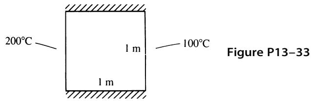
Figure P13–32 13.33 For the two-dimensional body shown in Figure P13–33, determine the temperature distribution. Let the left and right ends have constant temperatures of $2 0 0 ^ { \circ } \mathrm { C }$ and $1 0 0 ^ { \circ } \mathrm { C } .$ respectively. Let $K _ { x x } = K _ { y y } = 5 \ \mathbf { W } / ( \mathrm { m } \cdot ^ { \circ } \mathbf { C } )$ . The body is insulated along the top and bottom. 

text_image

200°C 1 m 1 m 100°C Figure P13-33

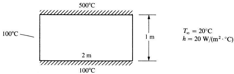
13.34 For the two-dimensional body shown in Figure P13–34, determine the temperature distribution. The top and bottom sides are insulated. The right side is subjected to heat transfer by convection. Let $K _ { x x } = K _ { y y } = 1 0 \mathrm { W } / ( \mathrm { m } \cdot ^ { \circ } \mathrm { C } )$ . 

text_image

500°C 100°C 2 m 100°C T∞ = 20°C h = 20 W/(m²·°C)

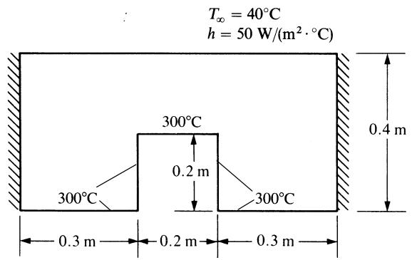
Figure P13–34 13.35 For the two-dimensional body shown in Figure P13–35, determine the temperature distribution. The left and right sides are insulated. The top surface is subjected to heat transfer by convection. The bottom and internal portion surfaces are maintained at $3 0 0 ^ { \circ } \mathrm { C } .$ 

text_image

T∞ = 40°C h = 50 W/(m²·°C) 300°C 300°C 0.2 m 300°C 0.3 m 0.2 m 0.3 m 0.4 m

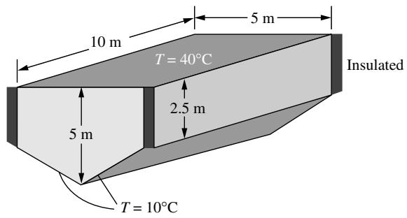
Figure P13–35 13.36 Determine the temperature distribution and rate of heat flow through the plain carbon steel ingot shown in Figure P13–36. Let $k = 6 0 \mathrm { W / m { - } K } )$ for the steel. The top surface is held at $4 0 ^ { \circ } \mathrm { C } ,$ while the underside surface is held at $0 ^ { \circ } \mathbf { C }$ . Assume that no heat is lost from the sides. 

text_image

10 m 5 m T = 40°C Insulated 2.5 m 5 m T = 10°C

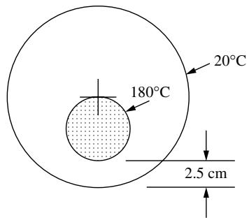
Figure P13–36 13.37 Determine the temperature distribution and rate of heat flow per foot length from a 5 cm outer diameter pipe at $1 8 0 ^ { \circ } \mathrm { C }$ placed eccentrically within a larger cylinder of insulation $( k = 0 . 0 5 8 \mathrm { W } / \mathrm { m } { \cdot } ^ { \circ } \mathrm { C } )$ as shown in Figure P13–37. The diameter of the outside cylinder is 15 cm, and the surface temperature is $2 0 ^ { \circ } \mathbf { C } .$ . 

text_image

20°C 180°C 2.5 cm

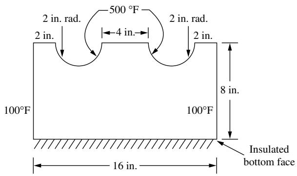
Figure P13–37  13.38 Determine the temperature distribution and rate of heat flow per foot length from the inner to the outer surface of the molded foam insulation $( k = 0 . 1 7 ~ \mathrm { B t u / h – f t – ^ { \circ } F } )$ shown in Figure P13–38.  

text_image

2 in. rad. 500 °F 2 in. rad. 2 in. 4 in. 2 in. 8 in. 100°F 100°F 16 in. Insulated bottom face

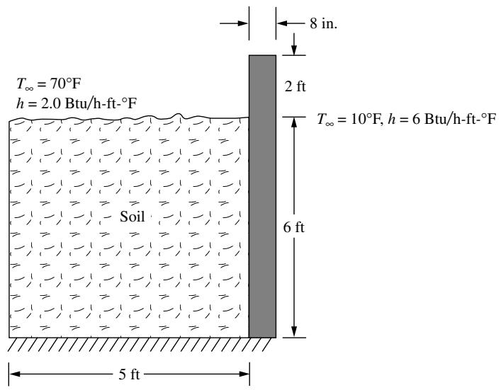
Figure P13–38 13.39 For the basement wall shown in Figure P13–39, determine the temperature distribution and the heat transfer through the wall and soil. The wall is constructed of concrete $( k = 1 . 0 ~ \mathrm { B t u / h – f t – ^ { \circ } F } )$ . The soil has an average thermal conductivity of $k = 0 . 8 5$ $\mathrm { B t u / h - f t - ^ { \circ } F }$ . The inside air is maintained at $7 0 ^ { \circ } \mathrm { F }$ with a convection coefficient $h = 2 . 0$ $\mathrm { B t u } / \mathrm { h } { - } \mathrm { f t } ^ { 2 } { - } ^ { \circ } \mathrm { F }$ . The outside air temperature is $1 0 ^ { \circ } \mathrm { F }$ with a heat transfer coefficient of $h = 6 \mathrm { \ B t u / h - f t ^ { 2 } - ^ { \circ } F }$ . Assume a reasonable distance from the wall of five feet that the horizontal component of heat transfer becomes negligible. Make sure this assumption is correct. 

text_image

T∞ = 70°F h = 2.0 Btu/h-ft-°F Soil 8 in. 2 ft T∞ = 10°F, h = 6 Btu/h-ft-°F 6 ft 5 ft

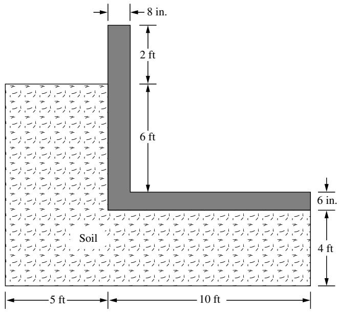
Figure P13–39 13.40 Now add a 6 in. thick concrete floor to the model of Figure P13–39 (as shown in Figure P13–40). Determine the temperature distribution and the heat transfer through the concrete and soil. Use the same properties as shown in P13–39.  

text_image

8 in. 2 ft 6 ft Soil 6 in. 4 ft 5 ft 10 ft

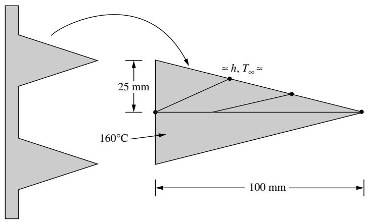
Figure P13–40 13.41 Aluminum fins $( k = 1 7 0 \mathrm { W / m { \mathrm { - } K } ) }$ with triangular profiles shown in Figure P13–41 are used to remove heat from a surface with a temperature of $1 6 0 ^ { \circ } \mathrm { C }$ . The temperature of the surrounding air is $2 5 ^ { \circ } \mathbf { C } .$ The natural convection coefficient is $h = 2 5 \mathrm { W / m ^ { 2 } { - } K }$ . Determine the temperature distribution throughout and the heat loss from a typical fin.  

text_image

25 mm 160°C ≈ h, T∞ ≈ 100 mm

Figure P13–41 13.42 Air is flowing at a rate of 10 lb/h inside a round tube with diameter of 1.5 in. and length of 10 in., similar to Figure 13–29 on page 572. The initial temperature of the air entering the tube is $5 0 ^ { \circ } \mathrm { F }$ . The wall of the tube has a uniform constant temperature of $2 0 0 ^ { \circ } \mathrm { F }$ . The specific heat of the air is 0.24 Btu/(lb-F), the convection coefficient between the air and the inner wall of the tube is $3 . 0 \ \mathrm { \ B t u } / ( \mathrm { h } { - } \mathrm { f t } ^ { 2 } { - } ^ { \circ } \mathrm { F } )$ , and the thermal conductivity is 0.017 Btu/(h-ft-F). Determine the temperature of the air along the length of the tube and the heat flow at the inlet and outlet of the tube.