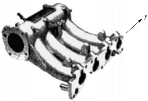
$( \alpha = 1 1 . 7 \times 1 0 ^ { - 6 } / { } ^ { \circ } \mathrm { C } )$ with a gasket separating the two materials. Assume a model as shown in Figure P15–9. If the temperature of the aluminum is increased by $4 0 ^ { \circ } \mathrm { C } ,$ what is the y displacement of the system and stress in each material? Also, what shear stress is induced in the bolted connection (assume two bolts in the connection)? Neglect the thin gasket in your model and assume the simplified model looks like Figure P15–11 below. 

natural_image

Mechanical component with multiple cylindrical cavities and a y-y coordinate arrow indicator (no text or symbols on the component itself)

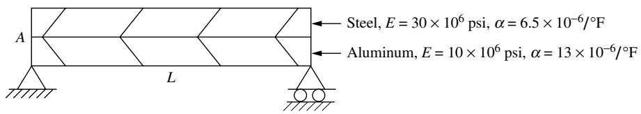
Figure P15–9 15.10 When do stresses occur in a body made of a single material due to uniform temperature change in the body? Consider problem 15.1 and also compare the solution to Example 15.1 in this chapter. 15.11 Consider two thermally incompatible materials, such as steel and aluminum, attached together as shown in Figure P15–11. Will there be temperature-induced stress in each material upon uniform heating of both materials to the same temperature when the boundary conditions are simple supports (a pin and a roller such that we have a statically determinate system)? Explain? Let there be a uniform temperature rise of $T = 5 0 ^ { \circ } \mathrm { F }$ . 

text_image

Steel, E = 30 × 10⁶ psi, α = 6.5 × 10⁻⁶/°F Aluminum, E = 10 × 10⁶ psi, α = 13 × 10⁻⁶/°F

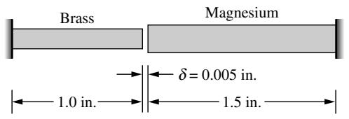
Figure P15–11 15.12 A bimetallic thermal control is made of a cold-rolled yellow brass and a magnesium alloy bar. The bars are arranged with a gap of 0.005 in. between them at $7 2 ^ { \circ } \mathrm { F }$ The brass bar has a length of 1.0 in. and a cross-sectional area of $0 . 1 0 \ { \mathrm { i n } } . ^ { 2 } { \mathrm { ; } }$ , and the magnesium bar has a length of 1.5 in. and a cross-sectional area of 0.15 in.2. Determine (a) the axial displacement of the end of the brass bar and (b) the stress in each bar after it has closed up due to a temperature increase of $1 0 0 ^ { \circ } \mathrm { F }$ . Use at least one element for each bar in your finite element model. 15.13 For the plane stress element shown in Figure P15–13 subjected to a uniform temperature rise of $T = 5 0 ^ { \circ } \mathrm { F }$ , determine the thermal force matrix $\{ f _ { T } \}$ . 

text_image

Brass Magnesium 1.0 in. 1.5 in. δ = 0.005 in.

Figure P15–12 

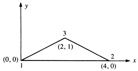
line

| Point | x | y | |---|---|---| | 1 | 0 | 0 | | 2 | 4 | 0 | | 3 | 2 | 1 |

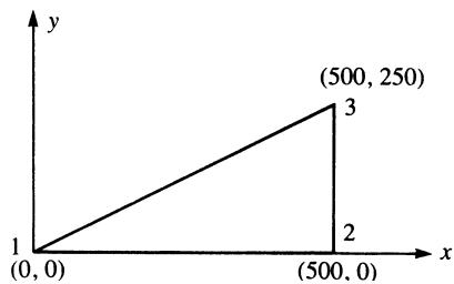
Figure P15–13 Let $E = 1 0 \times 1 0 ^ { 6 }$ psi, $\nu = 0 . 3 0$ , and $\alpha = 1 2 . 5 \times 1 0 ^ { - 6 } ~ ( \mathrm { i n . / i n . } ) / ^ { \circ } \mathrm { F }$ . The coordinates (in inches) are shown in the figure. The element thickness is t ¼ 1 in. 15.14 For the plane stress element shown in Figure P15–14 subjected to a uniform temperature rise of $T = 3 0 ^ { \circ } \mathrm { C }$ , determine the thermal force matrix $\{ f _ { T } \}$ . Let $E = 7 0 ~ \mathrm { G P a }$ , $\nu = 0 . 3 , \alpha = 2 3 \times 1 0 ^ { - 6 }$ (mm/mm)/ C, and t ¼ 5 mm. The coordinates (in millimeters) are shown in the figure. 

line

| x | y | |---|---| | 0 | 0 | | 500 | 250 | | 500 | 3 |

Figure P15–14 

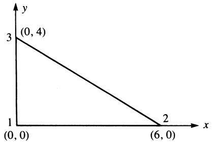
line

| x | y | |---|---| | 0 | 4 | | 6 | 0 |

Figure P15–15 15.15 For the plane stress element shown in Figure P15–15 subjected to a uniform temperature rise of $T = 1 0 0 ^ { \circ } \mathrm { { F } }$ , determine the thermal force matrix $\{ f _ { T } \}$ . Let $E = 3 0 \times 1 0 ^ { 6 }$ psi, $\nu = 0 . 3 , \alpha = 7 . 0 \times 1 0 ^ { - 6 } ( \mathrm { { i n } . \mathrm { { / i n } . ) / ^ { \circ } F _ { \mathrm { { } } } } }$ , and $t = 1$ in. The coordinates (in inches) are shown in the figure. 15.16 For the plane stress element shown in Figure P15–16 subjected to a uniform temperature drop of $T = 2 0 ^ { \circ } \mathrm { C }$ , determine the thermal force matrix $\{ f _ { T } \}$ . Let $E = 2 1 0 \mathrm { G P a }$ , $\nu = 0 . 2 5$ , and $\alpha = 1 2 \times 1 0 ^ { - 6 }$ $\mathrm { ( m m / m m ) / { } ^ { \circ } C }$ . The coordinates (in millimeters) are shown in the figure. The element thickness is 10 mm. 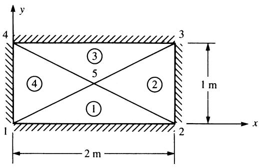15.17 For the plane stress plate fixed along the left and right sides and subjected to a uniform temperature rise of $5 0 ^ { \circ } \mathrm { F }$ as shown in Figure P15–17, determine the stresses in each element. Let $E = 1 0 \times 1 0 ^ { 6 } \mathrm { \ p s i } , \nu = 0 . 3 0 , \alpha = 1 2 . 5 \times 1 0 ^ { - 6 } \mathrm { ( i n . / i n . ) / } { } / { } ^ { \circ } \mathrm { F } .$ , and $\begin{array} { r } { t = \frac { 1 } { 4 } } \end{array}$ in. The coordinates (in inches) are shown in the figure. (Hint: The nodal displacements are all equal to zero. Therefore, the stresses can be determined from $\{ \sigma \} = - [ D ] \{ \varepsilon _ { T } \} . )$ （2号 

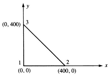
line

| Point | x | y | |---|---|---| | 1 | 0 | 0 | | 2 | 400 | 0 | | 3 | 0 | 400 |

Figure P15–16 

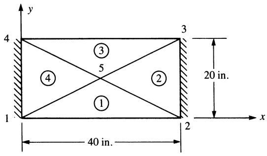
text_image

y 4 ③ 5 ④ ② ① 1 2 x 40 in. 20 in.

Figure P15–17 15.18 For the plane stress plate fixed along all edges and subjected to a uniform temperature decrease of $2 0 ^ { \circ } \mathrm { C }$ as shown in Figure P15–18, determine the stresses in each element. Let $E = 2 1 0 \mathrm { \ G P a } , \nu = 0 . 2 5 ,$ and $\alpha = 1 2 \times 1 0 ^ { - 6 }$ $( { \mathrm { m m / m m } } ) / { ^ { \circ } } \mathbf { C } .$ . The coordinates of the plate are shown in the figure. The plate thickness is 10 mm. (Hint: The nodal displacements are all equal to zero. Therefore, the stresses can be determined from $\{ \sigma \} = - [ D ] \{ \varepsilon _ { T } \} . )$ 

text_image

y 4 ③ 5 ② ④ ① 1 2 x 1 m 2 m 3

Figure P15–18 15.19 If the thermal expansion coefficient of a bar is given by $\alpha = \alpha _ { 0 } ( 1 + x / L )$ , determine the thermal force matrix. Let the bar have length $L ,$ modulus of elasticity $E ,$ and cross-sectional area A. 15.20 Assume the temperature function to vary linearly over the length of a bar as $T =$ $a _ { 1 } + a _ { 2 } x ;$ that is, express the temperature function as $\{ T \} = [ N ] \{ t \}$ , where $[ N ]$ is the shape function matrix for the two-node bar element. In other words, $[ N ] =$ $[ 1 - x / L \quad x / L ]$ . Determine the force matrix in terms of $E , A , \alpha , L , t _ { 1 }$ , and t2. [Hint: Use Eq. (15.1.18).] 15.21 Derive the thermal force matrix for the axisymmetric element of Chapter 9. (Also see Eq. (15.1.27).) # Using a computer program, solve the following problems. 15.22 The square plate in Figure P15–22 is subjected to uniform heating of $8 0 ^ { \circ } \mathrm { F }$ . Determine the nodal displacements and element stresses. Let the element thickness be $t = 0 . 1 \ \mathrm { i n } . , E = 3 0 \times 1 0 ^ { 6 } \ \mathrm { p s i } , \nu = 0 . 3 3 .$ , and $\alpha = 1 0 \times 1 0 ^ { - 6 } / { } ^ { \circ } \mathrm { F }$ . 

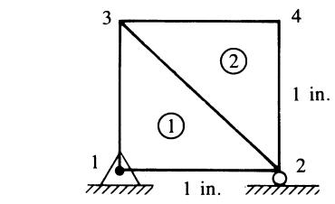
text_image

3 4 ② 1 in. ① 1 1 in. 2

Figure P15–22 

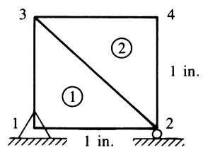
text_image

3 ② 1 in. ① 1 1 in. 2 4

Figure P15–23 15.23 The square plate in Figure P15–23 has element 1 made of steel with $E = 3 0 \times 1 0 ^ { 6 }$ psi, $\nu = 0 . 3 3$ , and $\alpha = 1 0 \times 1 0 ^ { - 6 } / { } ^ { \circ } \mathrm { F }$ and element 2 made of a material with $E = 1 5 \times 1 0 ^ { 6 }$ psi, $\nu = 0 . 2 5 ,$ , and $\alpha = 5 0 \times 1 0 ^ { - 6 } / { } ^ { \circ } \mathrm { F }$ . Let the plate thickness be $t = 0 . 1$ in. Determine the nodal displacements and element stresses for element 1 subjected to an 80 F temperature increase and element 2 subjected to a $5 0 ^ { \circ } \mathrm { F }$ temperature increase. 15.24 Solve Problem 15.3 using a computer program.  15.25 Solve Problem 15.6 using a computer program.  15.26 The aluminum tube shown in Figure P15–26 fits snugly into a hole at room temperature. If the temperature of the tube is then increased by $4 0 ^ { \circ } \mathrm { C } _ { ; }$ , determine the deformed configuration and the stress distribution of the tube. Let $E = 7 0 \ \mathrm { \ G P a }$ , $\nu = 0 . 3 3$ , and $\mathbf { \bar { \alpha } } \mathbf { \alpha } = 2 3 \times 1 0 ^ { - 6 } / ^ { \circ } \mathbf { C }$ for the tube. 

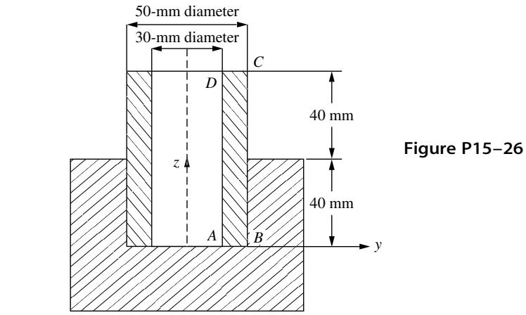
text_image

50-mm diameter 30-mm diameter C D z A B 40 mm 40 mm Figure P15-26 y

# Structural Dynamics and Time-Dependent Heat Transfer # Introduction This chapter provides an elementary introduction to time-dependent problems. We will introduce the basic concepts using the single-degree-of-freedom spring-mass system. We will include discussion of the stress analysis of the one-dimensional bar, beam, truss, and plane frame. This is followed by the analysis of one-dimensional heat transfer. We will provide the basic equations necessary for structural dynamics analysis and develop both the lumped- and the consistent-mass matrices involved in the analyses of the bar, beam, truss, and plane frame. We will describe the assembly of the global mass matrix for truss and plane frame analysis and then present numerical integration methods for handling the time derivative. We also present the mass matrices for the constant strain triangle and quadrilateral plane elements, for the axisymmetric element, and for the tetrahedral solid element. We will provide longhand solutions for the determination of the natural frequencies for bars and beams and then illustrate the time-step integration process involved with the stress analysis of a bar subjected to a time-dependent forcing function. We will next derive the basic equations for the time-dependent one-dimensional heat-transfer problem and discuss their applications. This chapter provides the basic concepts necessary for the solution of time-dependent problems. We conclude with a section on some computer program results for structural dynamics and time-dependent heat-transfer problems. 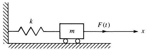# 16.1 Dynamics of a Spring-Mass System In this section, we discuss the motion of a single-degree-of-freedom spring-mass system to introduce the important concepts necessary for the later study of continuous systems such as bars, beams, and plane frames. In Figure 16–1, we show the 

text_image

k m F(t) x

Figure 16–1 Spring-mass system subjected to a time-dependent force single-degree-of-freedom spring-mass system subjected to a time-dependent force $F ( t )$ . Here k represents the spring stiffness or constant, and m represents the mass of the system. The free-body diagram of the mass is shown in Figure 16–2. The spring force $T = k x$ and the applied force $F ( t )$ act on the mass, and the mass-times-acceleration term is shown separately. Applying Newton’s second law of motion, $\mathbf { \boldsymbol { f } } = m \mathbf { \boldsymbol { a } } ,$ to the mass, we obtain the equation of motion in the x direction as $$ F (t) - k x = m \ddot {x} \tag {16.1.1} $$ where a dot over a variable denotes differentiation with respect to time; that is, $( \cdot ) = d ( ) / d t$ . Rewriting Eq. (16.1.1) in standard form, we have $$ m \ddot {x} + k x = F (t) \tag {16.1.2} $$ Equation (16.1.2) is a linear differential equation of the second order whose standard solution for the displacement x consists of a homogeneous solution and a particular solution. Standard analytical solutions for this forced vibration can be found in texts on dynamics or vibrations such as Reference [1]. The analytical solution will not be presented here as our intent is to introduce basic concepts in vibration behavior. However, we will solve the problem defined by Eq. (16.1.2) by an approximate numerical technique in Section 16.3 (see Examples 16.1 and 16.2). 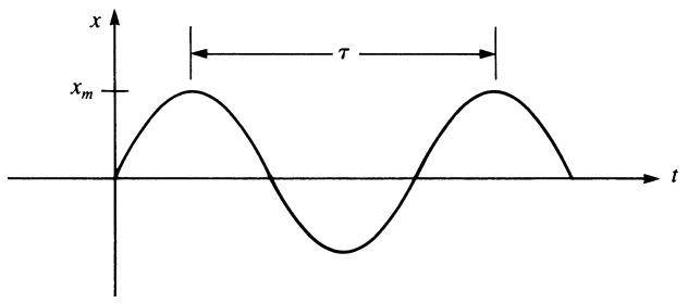The homogeneous solution to Eq. (16.1.2) is the solution obtained when the right side is set equal to zero. A number of useful concepts regarding vibrations are obtained by considering this free vibration of the mass—that is, when $F ( t ) = 0$ . Hence, defining $$ \omega^ {2} = \frac {k}{m} \tag {16.1.3} $$ and setting the right side of Eq. (16.1.2) equal to zero, we have $$ \ddot {x} + \omega^ {2} x = 0 \tag {16.1.4} $$ 

text_image

T = kx ← [ ] → F(t) = [ ] → ma = mdd

Figure 16–2 Free-body diagram of the mass of Figure 16–1 

text_image

x xₘ τ t

Figure 16–3 Displacement= time curve for simple harmonic motion where o is called the natural circular frequency of the free vibration of the mass, expressed in units of radians per second or revolutions per minute (rpm). Hence, the natural circular frequency defines the number of cycles per unit time of the mass vibration. We observe from Eq. (16.1.3) that o depends only on the spring stiffness k and the mass m of the body. The motion defined by Eq. (16.1.4) is called simple harmonic motion. The displacement and acceleration are seen to be proportional but of opposite direction. Again, a standard solution to Eq. (16.1.4) can be found in Reference [1]. A typical displacement/time curve is represented by the sine curve shown in Figure 16–3, where $x _ { m }$ denotes the maximum displacement (called the amplitude of the vibration). The time interval required for the mass to complete one full cycle of motion is called the period of the vibration t and is given by $$ \tau = \frac {2 \pi}{\omega} \tag {16.1.5} $$ where t is measured in seconds. Also the frequency in hertz $( { \mathrm { H } } z = 1 / { \mathrm { s } } )$ is $f =$ $1 / \tau = \omega / ( 2 \pi )$ . Finally, note that all vibrations are damped to some degree by friction forces. These forces may be caused by dry or Coulomb friction between rigid bodies, by internal friction between molecules within a deformable body, or by fluid friction when a body moves in a fluid. Damping results in natural circular frequencies that are smaller than those for undamped systems; maximum displacements also are smaller when damping occurs. A basic treatment of damping can be found in Reference [1] and additional discussion is included in Example 16.12. 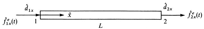# 16.2 Direct Derivation of the Bar Element Equations We will now derive the finite element equations for the time-dependent (dynamic) stress analysis of the one-dimensional bar. Recall that the time-independent (static) stress analysis of the bar was considered in Chapter 3. The steps used in deriving the dynamic equations are the same as those used for the derivation of the static equations. # Step 1 Select Element Type Figure 16–4 shows the typical bar element of length L, cross-sectional area $A ,$ and mass density r (with typical units of $\scriptstyle 1 6 - s ^ { 2 } / \mathrm { i n } ^ { 4 } )$ , with nodes 1 and 2 subjected to external time-dependent loads $\hat { f } _ { x } ^ { e } ( t )$ . 

text_image

f̂¹ˣᵗ(t) 1 x̂ L 2 d̂₁ˣ d̂₂ˣ f̂²ˣᵗ(t)

Figure 16–4 Bar element subjected to time-dependent loads # Step 2 Select a Displacement Function Again, we assume a linear displacement function along the x^ axis of the bar [see Eq. (3.1.1)]; that is, we let $$ \hat {u} = a _ {1} + a _ {2} \hat {x} \tag {16.2.1} $$ As was shown in Chapter 3, Eq. (16.2.1) can be expressed in terms of the shape functions as $$ \hat {u} = N _ {1} \hat {d} _ {1 x} + N _ {2} \hat {d} _ {2 x} \tag {16.2.2} $$ where $$ N _ {1} = 1 - \frac {\hat {x}}{L} \quad N _ {2} = \frac {\hat {x}}{L} \tag {16.2.3} $$ # Step 3 Define the Strain= Displacement and Stress=Strain Relationships Again, the strain/displacement relationship is given by $$ \{\varepsilon_ {x} \} = \frac {\partial \hat {u}}{\partial \hat {x}} = [ B ] \{\hat {d} \} \tag {16.2.4} $$ where $$ [ B ] = \left[ - \frac {1}{L} \quad \frac {1}{L} \right] \quad \{\hat {d} \} = \left\{ \begin{array}{l} \hat {d} _ {1 x} \\ \hat {d} _ {2 x} \end{array} \right\} \tag {16.2.5} $$ and the stress/strain relationship is given by $$ \{\sigma_ {x} \} = [ D ] \{\varepsilon_ {x} \} = [ D ] [ B ] \{\hat {d} \} \tag {16.2.6} $$ # Step 4 Derive the Element Stiffness and Mass Matrices and Equations The bar is generally not in equilibrium under a time-dependent force; hence, $f _ { 1 x } \neq$ $f _ { 2 x } .$ . Therefore, we again apply Newton’s second law of motion, $f = m \mathbf { { a } } ,$ , to each node. In general, the law can be written for each node as ‘‘the external (applied) force $f _ { x } ^ { e }$ minus the internal force is equal to the nodal mass times acceleration.’’ Equivalently, adding the internal force to the ma term, we have $$ \hat {f} _ {1 x} ^ {e} = \hat {f} _ {1 x} + m _ {1} \frac {\partial^ {2} \hat {d} _ {1 x}}{\partial t ^ {2}} \quad \hat {f} _ {2 x} ^ {e} = \hat {f} _ {2 x} + m _ {2} \frac {\partial^ {2} \hat {d} _ {2 x}}{\partial t ^ {2}} \tag {16.2.7} $$ where the masses $m _ { 1 }$ and $m _ { 2 }$ are obtained by lumping the total mass of the bar equally at the two nodes such that $$ m _ {1} = \frac {\rho A L}{2} \quad m _ {2} = \frac {\rho A L}{2} \tag {16.2.8} $$ In matrix form, we express Eqs. (16.2.7) as $$ \left\{ \begin{array}{l} \hat {f} _ {1 x} ^ {e} \\ \hat {f} _ {2 x} ^ {e} \end{array} \right\} = \left\{ \begin{array}{l} \hat {f} _ {1 x} \\ \hat {f} _ {2 x} \end{array} \right\} + \left[ \begin{array}{c c} m _ {1} & 0 \\ 0 & m _ {2} \end{array} \right] \left\{ \begin{array}{l} \frac {\partial^ {2} \hat {d} _ {1 x}}{\partial t ^ {2}} \\ \frac {\partial^ {2} \hat {d} _ {2 x}}{\partial t ^ {2}} \end{array} \right\} \tag {16.2.9} $$ Using Eqs. (3.1.13) and (3.1.14), we replace $\{ \hat { f } \}$ with $[ \hat { k } ] \{ \hat { d } \}$ in Eq. (16.2.9) to obtain the element equations $$ \{\hat {f} ^ {e} (t) \} = [ \hat {k} ] \{\hat {d} \} + [ \hat {m} ] \{\ddot {\hat {d}} \} \tag {16.2.10} $$ where $$ [ \hat {k} ] = \frac {A E}{L} \left[ \begin{array}{c c} 1 & - 1 \\ - 1 & 1 \end{array} \right] \tag {16.2.11} $$ is the bar element stiffness matrix, and $$ [ \hat {m} ] = \frac {\rho A L}{2} \left[ \begin{array}{l l} 1 & 0 \\ 0 & 1 \end{array} \right] \tag {16.2.12} $$ is called the lumped-mass matrix. Also, $$ \{\ddot {\hat {d}} \} = \frac {\partial^ {2} \{\hat {d} \}}{\partial t ^ {2}} \tag {16.2.13} $$ Observe that the lumped-mass matrix has diagonal terms only. This facilitates the computation of the global equations. However, solution accuracy is usually not as good as when a consistent-mass matrix is used [2]. We will now develop the consistent-mass matrix for the bar element. Numerous methods are available to obtain the consistent-mass matrix. The generally applicable virtual work principle (which is the basis of many energy principles, such as the principle of minimum potential energy for elastic bodies previously used in this text) provides a relatively simple method for derivation of the element equations and is included in Appendix E. However, an even simpler approach is to use D’Alembert’s principle; thus, we introduce an effective body force $X ^ { e }$ as $$ \{X ^ {e} \} = - \rho \{\ddot {\hat {u}} \} \tag {16.2.14} $$ where the minus sign is due to the fact that the acceleration produces D’Alembert’s body forces in the direction opposite the acceleration. The nodal forces associated with $\{ X ^ { e } \}$ are then found by using Eq. (6.3.1), repeated here as $$ \{f _ {b} \} = \iiint_ {V} [ N ] ^ {T} \{X \} d V \tag {16.2.15} $$ Substituting $\{ X ^ { e } \}$ given by Eq. (16.2.14) into Eq. (16.2.15) for $\{ X \}$ , we obtain $$ \left\{f _ {b} \right\} = - \iint_ {V} \rho [ N ] ^ {T} \{\ddot {u} \} d V \tag {16.2.16} $$ Recalling from Eq. (16.2.2) that $\{ \hat { u } \} = [ N ] \{ \hat { d } \}$ , we find that the first and second derivatives with respect to time are $$ \{\dot {\hat {u}} \} = [ N ] \{\dot {\hat {d}} \} \quad \{\ddot {\hat {u}} \} = [ N ] \{\ddot {\hat {d}} \} \tag {16.2.17} $$ where $\{ \dot { \hat { d } } \}$ and $\{ \ddot { \hat { d } } \}$ are the nodal velocities and accelerations, respectively. Substituting Eqs. (16.2.17) into Eq. (16.2.16), we obtain $$ \{f _ {b} \} = - \iint_ {V} \rho [ N ] ^ {T} [ N ] d V \{\ddot {\hat {d}} \} = - [ \hat {m} ] \{\ddot {\hat {d}} \} \tag {16.2.18} $$ where the element mass matrix is defined as $$ [ \hat {m} ] = \iint_ {V} \rho [ N ] ^ {T} [ N ] d V \tag {16.2.19} $$ This mass matrix is called the consistent-mass matrix because it is derived from the same shape functions ½N that are used to obtain the stiffness matrix $[ \hat { k } ]$ . In general, ½m^ given by Eq. (16.2.19) will be a full but symmetric matrix. Equation (16.2.19) is a general form of the consistent-mass matrix; that is, substituting the appropriate shape functions, we can generate the mass matrix for such elements as the bar, beam, and plane stress. We will now develop the consistent-mass matrix for the bar element of Figure 16–4 by substituting the shape function Eqs. (16.2.3) into Eq. (16.2.19) as follows: $$ [ \hat {m} ] = \iiint_ {V} \rho \left\{ \begin{array}{c} 1 - \frac {\hat {x}}{L} \\ \frac {\hat {x}}{L} \end{array} \right\} \left[ \begin{array}{l l} 1 - \frac {\hat {x}}{L} & \frac {\hat {x}}{L} \end{array} \right] d V \tag {16.2.20} $$ Simplifying Eq. (16.2.20), we obtain $$ [ \hat {m} ] = \rho A \int_ {0} ^ {L} \left\{ \begin{array}{c} 1 - \frac {\hat {x}}{L} \\ \frac {\hat {x}}{L} \end{array} \right\} \left[ \begin{array}{c c} 1 - \frac {\hat {x}}{L} & \frac {\hat {x}}{L} \end{array} \right] d \hat {x} \tag {16.2.21} $$