# Example For example, if a composite shell section were defined with the following input: ```csv *SHELL SECTION, COMPOSITE, NODAL THICKNESS, ELSET=name 1.5, 3, STEEL 2.5, 3, FOAM 1.0, 3, STEEL ``` and the total thickness at a point was only 1.0, the thicknesses of the individual layers at the point would be 0.3 for the first steel layer, 0.5 for the foam layer, and 0.2 for the second steel layer. # Creating a discontinuity in the shell, membrane, or rigid element thicknesses You can specify only a single thickness at each node. Therefore, use separate nodes along the interface on shell, membrane, or rigid elements where there is a discontinuity in the thickness and assign the appropriate thickness to each group of nodes. For elements that are not part of a rigid body, multi-point constraints must be used to make the displacements (and rotations, for shells) the same at corresponding nodes. # 2.1.4 NORMAL DEFINITIONS AT NODES Products: Abaqus/Standard Abaqus/Explicit # References • \*NORMAL • \*NODE # Overview Normals can be defined at nodes: • with a user-specified normal definition; • following the nodal coordinates as part of the node definition for beam and shell elements; • on rigid master surfaces used in contact pairs in Abaqus/Standard; • in beam and shell elements; • for line spring elements to give the direction normal to the flaw in the structure; • for gasket elements to give the thickness direction of the elements; and • for contour integral evaluation. The normals defined at nodes do not affect the element face normals, which are defined by the element connectivity. They need not be of unit length. # Contact surfaces in Abaqus/Standard User-specified surface normals for contact surfaces in Abaqus/Standard are relevant only when the smallsliding contact approach is used or when the finite-sliding contact approach is used with rigid elements that make up the master surface. User-specified surface normals defined on deformable master surfaces in contact pairs are ignored when finite sliding is used. The small-sliding contact formulation uses the surface normals at each node along the master surface to define a normal vector that varies smoothly from point to point on the surface. For a detailed discussion on how the “master plane” is constructed for each slave node using the surface normals, see “Contact formulations in Abaqus/Standard,” Section 38.1.1. For master surfaces composed of rigid elements Abaqus/Standard smooths any discontinuous surface normal transitions between the rigid elements. The surface normals at the nodes are used to control the surface normal interpolation. For a detailed discussion on the smoothing of such master surfaces, see “Analytical rigid surface definition,” Section 2.3.4. To define the normal, specify the components of the normal in the global coordinate system. Input File Usage: \*NORMAL, TYPE=CONTACT SURFACE # Elements User-specified normals may be necessary for beam and shell elements, line spring elements, gasket elements, or elements involved in contour integral evaluations. In such cases specify the components of the normal in the global coordinate system. Input File Usage: \*NORMAL, TYPE=ELEMENT # Beam and shell elements User-specified normals may be needed to define the desired normal directions at shell surface intersections or at beam intersections where the automatically determined normals may be inappropriate for the model (see “Beam element cross-section orientation,” Section 29.3.4, or “Defining the initial geometry of conventional shell elements,” Section 29.6.3). The nodal normals can also be defined as part of the node definition. While you can define a single normal for all elements connected to a node as part of the node definition, a user-specified normal definition defines a normal for a particular element at a node, thus allowing you to define separate normals for each element connected to a node. User-specified normal definitions supersede normals defined as part of a node definition. Input File Usage: \*NODE Specify the normals in the fifth, sixth, and seventh positions on the data line. For example, the following lines define some normals as part of node definitions; the normal to be used at node 7 in element 2 is then redefined using a user-specified normal definition: \*NODE 6, 5., 5., , -0.5, .8 7, 10., 8., , -0.5, .8 9, 14., 4., , .6, .6 \*NORMAL 2, 7, .6, .6 # Line spring elements For line spring elements user-specified normals can be used to give the direction normal to the flaw in the structure. See “Line spring elements for modeling part-through cracks in shells,” Section 32.9.1, for a description of these elements. # Gasket elements For gasket elements user-specified normals can be used to specify the thickness direction of the elements. The nodal thickness directions can also be defined as part of the gasket section definition. Thickness directions defined by user-specified normals supersede thickness directions defined as part of the gasket section definition. See “Defining the gasket element’s initial geometry,” Section 32.6.4, for a description of the definition of the thickness direction for these elements. # Contour integral evaluation For contour integral evaluations (“Contour integral evaluation,” Section 11.4.2) surface normals should be specified at all surface nodes lying within the bounds of the requested contours. These nodes are printed out under the “Contour Integral” information in the data (.dat) file. For accurate contour integral evaluation it is important that the virtual crack extension direction is in the plane of the surface for the following cases: when a crack front intersects the external surface of a three-dimensional solid, when the crack front intersects a surface of material discontinuity, or when the crack is in a curved shell. If no normals are specified, Abaqus will calculate the normals automatically. The nodal normal data specified as part of a node definition will not be activated for solid elements unless a user-specified normal definition is used in the model; it suffices to include a user-specified normal definition for only one node to activate the utilization of the nodal normal data specified as part of a node definition. # The coordinate system in which normals are defined Abaqus models can be defined in terms of an assembly of part instances (see “Defining an assembly,” Section 2.10.1). Normals at nodes defined within a part (or part instance) are defined relative to the part coordinate system. These normals are rotated according to the positioning data given for each instance of the part. Normals can be defined at reference nodes at the assembly level if necessary. Normals defined at the assembly level are defined in the global coordinate system. For models that are not defined in terms of an assembly of part instances, normals are defined in the global coordinate system. # 2.1.5 TRANSFORMED COORDINATE SYSTEMS Products: Abaqus/Standard Abaqus/Explicit Abaqus/CAE # References • “Prescribed conditions: overview,” Section 34.1.1 • \*TRANSFORM • “Transforming results into a new coordinate system,” Section 42.6.8 of the Abaqus/CAE User’s Guide, in the HTML version of this guide • “An overview of the methods for creating a datum coordinate system,” Section 62.5.4 of the Abaqus/CAE User’s Guide # Overview A nodal transformation is used to define a local coordinate system for: • the definition of concentrated forces and moments; • the definition of displacement and rotation boundary conditions; • the definition of linear constraint equations; and • the output of vector-valued quantities. A nodal transformation cannot be used to specify a local coordinate system for defining: • nodal coordinates—see “Specifying a local coordinate system in which to define nodes” in “Node definition,” Section 2.1.1, or “Specifying a local coordinate system for the nodal coordinates” in “Node definition,” Section 2.1.1, instead; or • material properties or rebars—see “Orientations,” Section 2.2.5, instead. # Defining a local coordinate system Normally displacement and rotation components are associated with the global, rectangular Cartesian axis system. When a transformed coordinate system is associated with a node, all input data for concentrated forces and moments and for displacement and rotation boundary conditions at the node are given in the local system. The following transformations are available: • Rectangular Cartesian • Cylindrical • Spherical The coordinate transformation defined at a node must be consistent with the degrees of freedom that exist at the node. For example, a transformed coordinate system should not be defined at a node that is connected only to a SPRING1 or SPRING2 element, since these elements have only one active degree of freedom per node.

Input File Usage:	You must identify the node set for which the local transformed system is defined.
	*TRANSFORM, NSET=name
Abaqus/CAE Usage:	In Abaqus/CAE you define a local coordinate system independent of its use and then refer to it when you apply a load or boundary condition at a node.
	Any module:Tools→Datum:Type:CSYS
	Interaction module: load or boundary condition editor:CSYS:Edit:select local coordinate system

# Defining a local coordinate system in a model that contains an assembly of part instances In a model defined in terms of an assembly of part instances, you can define a nodal transformation at the part, part instance, or assembly level. A nodal transformation defined at the part or part instance level will be rotated according to the positioning data given for each instance of that part (or for the part instance). See “Defining an assembly,” Section 2.10.1. Multiple transformation definitions are not allowed at a node, even if one of them is at the part level and another is at the assembly level. # Large-displacement analysis The transformed coordinate system is always a set of fixed Cartesian axes at a node (even for cylindrical or spherical transforms). These transformed directions are fixed in space; the directions do not rotate as the node moves. Therefore, even in large-displacement analysis, the displacement components must always be given with respect to these fixed directions in space. 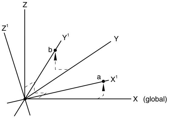# Defining a rectangular Cartesian coordinate transformation In a rectangular Cartesian transformation the transformed directions are parallel at all nodes of the set. The coordinates of two points must be given, as shown in Figure 2.1.5–1. 

text_image

Z Z¹ Y¹ b Y a X¹ X (global)

Figure 2.1.5–1 Cartesian transformation. The first point, a, must be on a line through the global origin; this point defines the transformed $X ^ { 1 }$ -direction. The second point, b, must be in the plane containing the global origin and the transformed $X ^ { 1 }$ - and $Y ^ { 1 }$ -directions. This second point should be on or near the positive $Y ^ { 1 } { \mathrm { - a x i s } }$ . Input File Usage: \*TRANSFORM, NSET=name, TYPE=R (default) Abaqus/CAE Usage: Any module: Tools→Datum: Type: CSYS: select any method, and click OK: Rectangular # Defining a cylindrical coordinate transformation The radial, tangential, and axial directions must be defined based on the original coordinates of each node in the node set for which the transformation is invoked. The global $( X , Y , Z )$ coordinates of the two points defining the axis of the cylindrical system (points a and b as shown in Figure 2.1.5–2) must be given. 

text_image

Z Y X (global) (a radial) X¹ (axial) Z¹ b a Y¹ (tangential)

Figure 2.1.5–2 Cylindrical transformation. The origin of the local coordinate system is at the node of interest. The local $X ^ { 1 }$ -axis is defined by a line through the node, perpendicular to the line through points a and b. The local $Z ^ { 1 }$ -axis is defined by a line that is parallel to the line through points a and b. The local $Y ^ { 1 }$ -axis forms a right-handed coordinate system with $X ^ { 1 }$ and $Z ^ { 1 }$ . A cylindrical coordinate system cannot be defined for a node that lies along the line joining points a and b. Input File Usage: \*TRANSFORM, NSET=name, TYPE=C Abaqus/CAE Usage: Any module: Tools→Datum: Type: CSYS: select any method, and click OK: Cylindrical # Defining a spherical coordinate transformation The radial, circumferential, and meridional directions must be defined based on the original coordinates of each node in the node set for which the transformation is invoked. The global $( X , Y , Z )$ coordinates of the center of the spherical system, a, and of a point on the polar axis, b, must be given as shown in Figure 2.1.5–3. 

text_image

Z Y X (global) b Z¹ (meridional) a Y¹ (circumferential) X¹ (radial)

Figure 2.1.5–3 Spherical transformation. The origin of the local coordinate system is at the node of interest. The local $X ^ { 1 }$ -axis is defined by a line through the node and point a. The local $Z ^ { 1 }$ -axis lies in a plane containing the polar axis (the line between points a and b) and is perpendicular to the local $X ^ { 1 }$ -axis. The local $Y ^ { 1 }$ -axis forms a right-handed coordinate system with $X ^ { 1 }$ and $Z ^ { 1 }$ . A spherical coordinate system cannot be defined for a node that lies along the line joining points a and b. Input File Usage: \*TRANSFORM, NSET=name, TYPE=S Abaqus/CAE Usage: Any module: Tools→Datum: Type: CSYS: select any method, and click OK: Spherical # Output at a node associated with a coordinate transformation Printed and file output of vector-valued quantities from Abaqus/Standard at transformed nodes can be in the local or global system (see “Specifying the directions for nodal output” in “Output to the data and results files,” Section 4.1.2). By default, the values are written to the data file in the local system, whereas the values are written to the results file in the global system (since this is more convenient for postprocessing). Consequently, reaction forces printed using the default will not appear to equilibrate loads applied in the global system. However, these reaction forces and loads should equilibrate if you output them to the data file in the global system. File output from Abaqus/Explicit is always in the global system. Output database output of field vector-valued quantities at transformed nodes is in the global system. The local transformations are also written to the output database. You can apply these transformations to