```c *BOUNDARY, AMPLITUDE=name Data lines to describe zero-valued or nonzero boundary conditions *CLOAD and/or *DLOAD Data lines to specify loads *TEMPERATURE and/or *FIELD Data lines to specify values of predefined fields *END STEP ** *STEP *ANNEAL (,TEMPERATURE=θ) *END STEP ** *STEP *DYNAMIC, EXPLICIT (,ADIABATIC) Data line to specify the time period of the step *BOUNDARY, AMPLITUDE=name Data lines to describe zero-valued or nonzero boundary conditions *CLOAD and/or *DLOAD and/or *DSLOAD Data lines to specify loads *TEMPERATURE and/or *FIELD Data lines to specify values of predefined fields *END STEP ``` # 7. Analysis Solution and Control Solving nonlinear problems 7.1 Analysis convergence controls 7.2 # 7.1 Solving nonlinear problems • “Solving nonlinear problems,” Section 7.1.1 # 7.1.1 SOLVING NONLINEAR PROBLEMS Products: Abaqus/Standard Abaqus/CAE # References • “Convergence and time integration criteria: overview,” Section 7.2.1 • “Commonly used control parameters,” Section 7.2.2 • “Convergence criteria for nonlinear problems,” Section 7.2.3 • “Time integration accuracy in transient problems,” Section 7.2.4 • “Configuring general analysis procedures,” Section 14.11.1 of the Abaqus/CAE User’s Guide, in the HTML version of this guide # Overview Solving nonlinear problems in Abaqus/Standard involves: • a combination of incremental and iterative procedures; • using the Newton method to solve the nonlinear equations; • determining convergence; • defining loads as a function of time; and • choosing suitable time increments automatically. Some static problems may become unstable because of severe nonlinearity. Abaqus/Standard offers a set of automatic stabilization mechanisms to handle such problems. 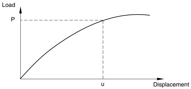# The solution of nonlinear problems The nonlinear load-displacement curve for a structure is shown in Figure 7.1.1–1. 

line

| Displacement | Load | | ------------ | ---- | | 0 | 0 | | u | P |

Figure 7.1.1–1 Nonlinear load-displacement curve. The objective of the analysis is to determine this response. In a nonlinear analysis the solution cannot be calculated by solving a single system of linear equations, as would be done in a linear problem. Instead, the solution is found by specifying the loading as a function of time and incrementing time to obtain the nonlinear response. Therefore, Abaqus/Standard breaks the simulation into a number of time increments and finds the approximate equilibrium configuration at the end of each time increment. Using the Newton method, it often takes Abaqus/Standard several iterations to determine an acceptable solution to each time increment. # Steps, increments, and iterations • The time history for a simulation consists of one or more steps. You define the steps, which generally consist of an analysis procedure, loading, and output requests. Different loads, boundary conditions, analysis procedures, and output requests can be used in each step. For example: Step 1: Hold a plate between rigid jaws. Step 2: Add loads to deform the plate. Step 3: Find the natural frequencies of the deformed plate. • An increment is part of a step. In nonlinear analyses each step is broken into increments so that the nonlinear solution path can be followed. You suggest the size of the first increment, and Abaqus/Standard automatically chooses the size of the subsequent increments. At the end of each increment the structure is in (approximate) equilibrium and results are available for writing to the restart, data, results, or output database files. • An iteration is an attempt at finding an equilibrium solution in an increment. If the model is not in equilibrium at the end of the iteration, Abaqus/Standard tries another iteration. With every iteration the solution that Abaqus/Standard obtains should be closer to equilibrium; however, sometimes the iteration process may diverge—subsequent iterations may move away from the equilibrium state. In that case Abaqus/Standard may terminate the iteration process and attempt to find a solution with a smaller increment size. 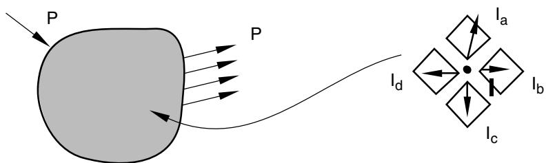# Convergence Consider the external forces, P, and the internal (nodal) forces, I, acting on a body (see Figure 7.1.1–2(a) and Figure 7.1.1–2(b), respectively). The internal loads acting on a node are caused by the stresses in the elements that are attached to that node. For the body to be in equilibrium, the net force acting at every node must be zero. Therefore, the basic statement of equilibrium is that the internal forces, I, and the external forces, P, must balance each other: $$ P - I = 0. 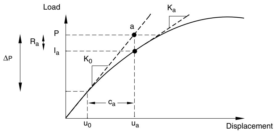$$ The nonlinear response of a structure to a small load increment, $\Delta P$ , is shown in Figure 7.1.1–3. Abaqus/Standard uses the structure’s tangent stiffness, $K _ { 0 }$ , which is based on its configuration at $u _ { 0 }$ , and $\Delta P$ to calculate a displacement correction, $c _ { a }$ , for the structure. Using $c _ { a }$ , the structure’s configuration is updated to $u _ { a }$ . 

text_image

P P Id Ia Ib Ic

(a) External loads in a simulation. (b) Internal forces acting at a node. Figure 7.1.1–2 Internal and external loads on a body. 

line

| Displacement | Load | Label | | ------------ | ---- | ----- | | u₀ | P | a | | uₐ | P | K₀ | | uₐ | Iₐ | Iₐ | | uₐ | Kₐ | Kₐ |

Figure 7.1.1–3 First iteration in an increment. Abaqus/Standard then calculates the structure’s internal forces, $I _ { a }$ , in this updated configuration. The difference between the total applied load, P, and $I _ { a }$ can now be calculated as $$ R _ {a} = P - I _ {a}, $$ where $R _ { a }$ is the force residual for the iteration. If $R _ { a }$ is zero at every degree of freedom in the model, point a in Figure 7.1.1–3 would lie on the load-deflection curve and the structure would be in equilibrium. In a nonlinear problem $R _ { a }$ will never be exactly zero, so Abaqus/Standard compares it to a tolerance value. If $R _ { a }$ is less than this force residual tolerance at all nodes, Abaqus/Standard accepts the solution as being in equilibrium. By default, this tolerance value is set to 0.5% of an average force in the structure, averaged over time. Abaqus/Standard automatically calculates this spatially and time-averaged force throughout the simulation. You can change this, and all other such tolerances, by specifying solution controls (see “Convergence criteria for nonlinear problems,” Section 7.2.3). If $R _ { a }$ is less than the current tolerance value, P and $I _ { a }$ are considered to be in equilibrium and $u _ { a }$ is a valid equilibrium configuration for the structure under the applied load. However, before Abaqus/Standard accepts the solution, it also checks that the last displacement correction, $c _ { a }$ , is small relative to the total incremental displacement, $\Delta u _ { a } = u _ { a } - u _ { 0 }$ . If $c _ { a }$ is greater than a fraction (1% by default) of the incremental displacement, Abaqus/Standard performs another iteration. Both convergence checks must be satisfied before a solution is said to have converged for that time increment. 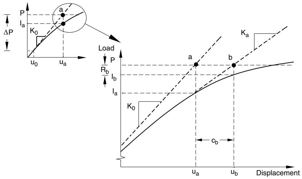If the solution from an iteration is not converged, Abaqus/Standard performs another iteration to try to bring the internal and external forces into balance. First, Abaqus/Standard forms the new stiffness, $K _ { a } ,$ , for the structure based on the updated configuration, $u _ { a }$ . This stiffness, together with the residual $R _ { a }$ , determines another displacement correction, $c _ { b }$ , that brings the system closer to equilibrium (point b in Figure 7.1.1–4). 

line

| Point | Load (P) | Displacement (u_a) | Displacement (u_b) | |-------|----------|---------------------|---------------------| | a | K₀ | ~0.5 | ~0.5 | | b | K₀ | ~0.5 | ~0.5 |

Figure 7.1.1–4 Second iteration. Abaqus/Standard calculates a new force residual, $R _ { b }$ , using the internal forces from the structure’s new configuration, $u _ { b }$ . Again, the largest force residual at any degree of freedom, $R _ { b }$ , is compared against the force residual tolerance, and the displacement correction for the second iteration, $c _ { b } .$ , is compared to the increment of displacement, $\Delta u _ { b }$ . If necessary, Abaqus/Standard performs further iterations. For more details on convergence in Abaqus/Standard, see “Convergence criteria for nonlinear problems,” Section 7.2.3. For each iteration in a nonlinear analysis Abaqus/Standard forms the model’s stiffness matrix and solves a system of equations. Therefore, the computational cost of each iteration is close to the cost of conducting a complete linear analysis, making the computational expense of a nonlinear