$$ \left\{ \begin{array}{l} t _ {n} \\ t _ {s} \\ t _ {t} \end{array} \right\} = \left[ \begin{array}{c c c} E _ {n n} & & \\ & E _ {s s} & \\ & & E _ {t t} \end{array} \right] \left\{ \begin{array}{l} \varepsilon_ {n} \\ \varepsilon_ {s} \\ \varepsilon_ {t} \end{array} \right\}. $$ The quantities $t _ { n } , \ t _ { s }$ , and $t _ { t }$ represent the nominal tractions in the normal and the two local shear directions, respectively; while the quantities $\varepsilon _ { n } , \varepsilon _ { s }$ , and $\varepsilon _ { t }$ represent the corresponding nominal strains. For coupled traction separation behavior the stress-strain relations are as follows: $$ \left\{ \begin{array}{l} t _ {n} \\ t _ {s} \\ t _ {t} \end{array} \right\} = \left[ \begin{array}{c c c} E _ {n n} & E _ {n s} & E _ {n t} \\ E _ {n s} & E _ {s s} & E _ {s t} \\ E _ {n t} & E _ {s t} & E _ {t t} \end{array} \right] \left\{ \begin{array}{l} \varepsilon_ {n} \\ \varepsilon_ {s} \\ \varepsilon_ {t} \end{array} \right\}. $$ Input File Usage: Use the following option to define uncoupled elastic behavior for cohesive elements: \*ELASTIC, TYPE=TRACTION Use the following option to define coupled elastic behavior for cohesive elements: \*ELASTIC, TYPE=COUPLED TRACTION Abaqus/CAE Usage: Use the following option to define uncoupled elastic behavior for cohesive elements: Property module: material editor: Mechanical→Elasticity→Elastic: # Type: Traction Use the following option to define coupled elastic behavior for cohesive elements: Property module: material editor: Mechanical→Elasticity→Elastic: # Type: Coupled Traction # Stability The stability criterion for uncoupled behavior requires that $E _ { n n } > 0 , E _ { s s } > 0$ , and $E _ { t t } > 0$ . For coupled behavior the stability criterion requires that: $$ E _ {n n} > 0, \quad E _ {s s} > 0, \quad E _ {t t} > 0; $$ $$ E _ {n s} < \sqrt {E _ {n n} E _ {s s}}; $$ $$ E _ {s t} < \sqrt {E _ {s s} E _ {t t}}; $$ $$ E _ {n t} < \sqrt {E _ {n n} E _ {t t}}; $$ $$ d e t \left[ \begin{array}{c c c} E _ {n n} & E _ {n s} & E _ {n t} \\ E _ {n s} & E _ {s s} & E _ {s t} \\ E _ {n t} & E _ {s t} & E _ {t t} \end{array} \right] > 0. $$ # Defining isotropic shear elasticity for equations of state in Abaqus/Explicit Abaqus/Explicit allows you to define isotropic shear elasticity to describe the deviatoric response of materials whose volumetric response is governed by an equation of state (“Elastic shear behavior” in “Equation of state,” Section 25.2.1). In this case the deviatoric stress-strain relationship is given by $$ \mathbf {S} = 2 \mu \mathbf {e} ^ {e l}, $$ where is the deviatoric stress and $\mathbf { e } ^ { e l }$ is the deviatoric elastic strain. You must provide the elastic shear modulus, $\mu ,$ when you define the elastic deviatoric behavior. Input File Usage: \*ELASTIC, TYPE=SHEAR Abaqus/CAE Usage: Property module: material editor: Mechanical→Elasticity→Elastic: Type: Shear # Elements Linear elasticity can be used with any stress/displacement element or coupled temperature-displacement element in Abaqus. The exceptions are traction elasticity, which can be used only with warping elements and cohesive elements; coupled traction elasticity, which can be used only with cohesive elements; shear elasticity, which can be used only with solid (continuum) elements except plane stress elements; and, in Abaqus/Explicit, anisotropic elasticity, which is not supported for truss, rebar, pipe, and beam elements. If the material is (almost) incompressible (Poisson’s ratio $\nu > 0 . 4 9$ for isotropic elasticity), hybrid elements should be used in Abaqus/Standard. Compressible anisotropic elasticity should not be used with second-order hybrid continuum elements: inaccurate results and/or convergence problems may occur. # 22.2.2 NO COMPRESSION OR NO TENSION Products: Abaqus/Standard Abaqus/CAE WARNING: Except when used with truss or beam elements, Abaqus/Standard does not form an exact material stiffness for this option. Therefore, the convergence can sometimes be slow. # References • “Material library: overview,” Section 21.1.1 • “Elastic behavior: overview,” Section 22.1.1 • “Linear elastic behavior,” Section 22.2.1 • \*NO COMPRESSION • \*NO TENSION • “Specifying elastic material properties” in “Defining elasticity,” Section 12.9.1 of the Abaqus/CAE User’s Guide, in the HTML version of this guide # Overview The no compression and no tension elasticity models: • are used to modify the linear elasticity of the material so that compressive stress or tensile stress cannot be generated; and • can be used only in conjunction with an elasticity definition. # Defining the modified elastic behavior The modified elastic behavior is obtained by first solving for the principal stresses assuming linear elasticity and then setting the appropriate principal stress values to zero. The associated stiffness matrix components will also be set to zero. These models are not history dependent: the directions in which the principal stresses are set to zero are recalculated at every iteration. The no compression effect for a one-dimensional stress case such as a truss or a layer of a beam in a plane is illustrated in Figure 22.2.2–1. No compression and no tension definitions modify only the elastic response of the material.  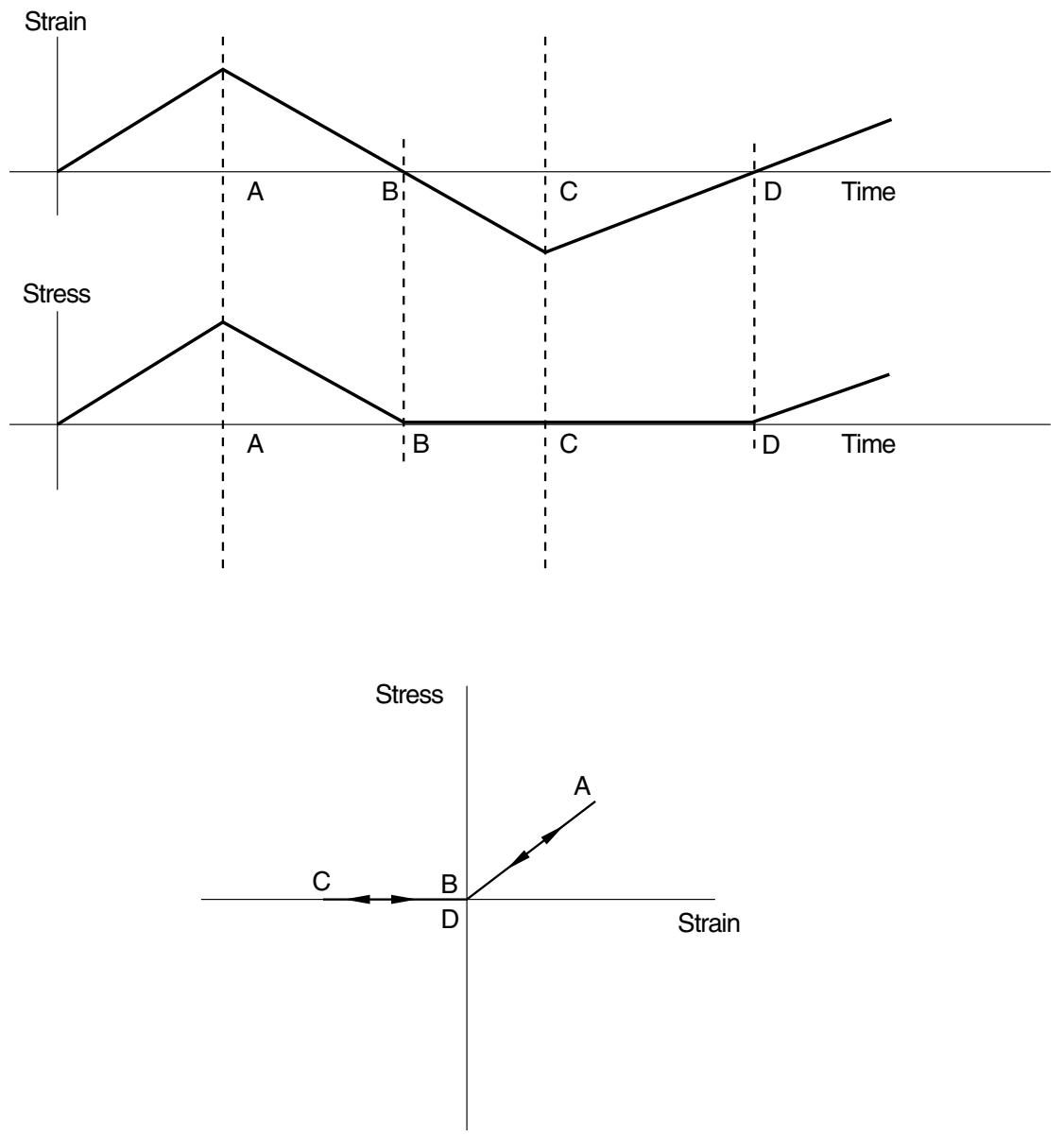Figure 22.2.2–1 A no compression elastic case with an imposed strain cycle. Input File Usage: Use one of the following options: \*NO COMPRESSION \*NO TENSION # Abaqus/CAE Usage: Property module: material editor: Mechanical→Elasticity→Elastic: No compression or No tension # Stability Using no compression or no tension elasticity can make a model unstable: convergence difficulties may occur. Sometimes these difficulties can be overcome by overlaying each element that uses the no compression (or no tension) model with another element that uses a small value of Young’s modulus (small in comparison with the Young’s modulus of the element using modified elasticity). This technique creates a small “artificial” stiffness, which can stabilize the model. # Use with other material models No compression and no tension definitions can be used only in conjunction with an elasticity definition. These definitions cannot be used with any other material option. # Elements The no compression and no tension elasticity models can be used with any stress/displacement element in Abaqus/Standard. However, they cannot be used with shell elements or beam elements if section properties are pre-integrated using a general section definition. # 22.2.3 PLANE STRESS ORTHOTROPIC FAILURE MEASURES Products: Abaqus/Standard Abaqus/Explicit Abaqus/CAE # References • “Material library: overview,” Section 21.1.1 • “Elastic behavior: overview,” Section 22.1.1 • “Linear elastic behavior,” Section 22.2.1 • \*FAIL STRAIN • \*FAIL STRESS • \*ELASTIC • “Defining stress-based failure measures for an elastic model” in “Defining elasticity,” Section 12.9.1 of the Abaqus/CAE User’s Guide, in the HTML version of this guide • “Defining strain-based failure measures for an elastic model” in “Defining elasticity,” Section 12.9.1 of the Abaqus/CAE User’s Guide, in the HTML version of this guide # Overview The orthotropic plane stress failure measures: • are indications of material failure (normally used for fiber-reinforced composite materials; for alternative damage and failure models for fiber-reinforced composite materials, see “Damage and failure for fiber-reinforced composites: overview,” Section 24.3.1); • can be used only in conjunction with a linear elastic material model (with or without local material orientations); • can be used for any element that uses a plane stress formulation; that is, for plane stress continuum elements, shell elements, and membrane elements; • are postprocessed output requests and do not cause any material degradation; and • take values that are greater than or equal to 0.0, with values that are greater than or equal to 1.0 implying failure. # Failure theories Five different failure theories are provided: four stress-based theories and one strain-based theory. We denote orthotropic material directions by 1 and 2, with the 1-material direction aligned with the fibers and the 2-material direction transverse to the fibers. For the failure theories to work correctly, the 1- and 2-directions of the user-defined elastic material constants must align with the fiber and the transverseto-fiber directions, respectively. For applications other than fiber-reinforced composites, the 1- and 2- material directions should represent the strong and weak orthotropic-material directions, respectively. In all cases tensile values must be positive and compressive values must be negative. The input data for the stress-based failure theories are tensile and compressive stress limits, $X _ { t }$ and $X _ { c }$ , in the 1-direction; tensile and compressive stress limits, $Y _ { t }$ and $Y _ { c } ,$ in the 2-direction; and shear strength (maximum shear stress), ${ \cal S } ,$ in the $X { - } Y$ plane. All four stress-based theories are defined and available with a single definition in Abaqus; the desired output is chosen by the output variables described at the end of this section. Input File Usage: \*FAIL STRESS Abaqus/CAE Usage: Property module: material editor: Mechanical→Elasticity→Elastic: Suboptions→Fail Stress # Maximum stress theory If $\sigma _ { 1 1 } > 0 , X = X _ { t } ; $ otherwise, $X = X _ { c }$ . If $\sigma _ { 2 2 } > 0 , Y = Y _ { t }$ ; otherwise, $Y = Y _ { c }$ . The maximum stress failure criterion requires that $$ I _ {F} = \max \left(\frac {\sigma_ {1 1}}{X}, \frac {\sigma_ {2 2}}{Y}, \left| \frac {\sigma_ {1 2}}{S} \right|\right) < 1. 0. $$ # Tsai-Hill theory $\operatorname { I f } \sigma _ { 1 1 } > 0 , X = X _ { t } ;$ otherwise, $X = X _ { c } . { \mathrm { ~ I f ~ } } \sigma _ { 2 2 } > 0 , Y = Y _ { t }$ ; otherwise, $Y = Y _ { c }$ . The Tsai-Hill failure criterion requires that $$ I _ {F} = \frac {\sigma_ {1 1} ^ {2}}{X ^ {2}} - \frac {\sigma_ {1 1} \sigma_ {2 2}}{X ^ {2}} + \frac {\sigma_ {2 2} ^ {2}}{Y ^ {2}} + \frac {\sigma_ {1 2} ^ {2}}{S ^ {2}} < 1. 0. $$ # Tsai-Wu theory The Tsai-Wu failure criterion requires that $$ I _ {F} = F _ {1} \sigma_ {1 1} + F _ {2} \sigma_ {2 2} + F _ {1 1} \sigma_ {1 1} ^ {2} + F _ {2 2} \sigma_ {2 2} ^ {2} + F _ {6 6} \sigma_ {1 2} ^ {2} + 2 F _ {1 2} \sigma_ {1 1} \sigma_ {2 2} < 1. 0. $$ The Tsai-Wu coefficients are defined as follows: $$ F _ {1} = \frac {1}{X _ {t}} + \frac {1}{X _ {c}}, \quad F _ {2} = \frac {1}{Y _ {t}} + \frac {1}{Y _ {c}}, \quad F _ {1 1} = - \frac {1}{X _ {t} X _ {c}}, \quad F _ {2 2} = - \frac {1}{Y _ {t} Y _ {c}}, \quad F _ {6 6} = \frac {1}{S ^ {2}}. $$ $\sigma _ { b i a x }$ is the equibiaxial stress at failure. If it is known, then $$ F _ {1 2} = \frac {1}{2 \sigma_ {b i a x} ^ {2}} \left[ 1 - \left(\frac {1}{X _ {t}} + \frac {1}{X _ {c}} + \frac {1}{Y _ {t}} + \frac {1}{Y _ {c}}\right) \sigma_ {b i a x} + \left(\frac {1}{X _ {t} X _ {c}} + \frac {1}{Y _ {t} Y _ {c}}\right) \sigma_ {b i a x} ^ {2} \right]; $$ otherwise, $$ F _ {1 2} = \stackrel {*} {f} \sqrt {F _ {1 1} F _ {2 2}}, $$ where $- 1 . 0 \leq \stackrel { * } { f } \leq 1 . 0$ . The default value of $\stackrel { * } { f }$ is zero. For the Tsai-Wu failure criterion either $\stackrel { * } { f }$ or $\sigma _ { b i a x }$ must be given as input data. The coefficient $\stackrel { * } { f }$ is ignored if $\sigma _ { b i a x }$ is given. # Azzi-Tsai-Hill theory The Azzi-Tsai-Hill failure theory is the same as the Tsai-Hill theory, except that the absolute value of the cross product term is taken: $$ I _ {F} = \frac {\sigma_ {1 1} ^ {2}}{X ^ {2}} - \frac {| \sigma_ {1 1} \sigma_ {2 2} |}{X ^ {2}} + \frac {\sigma_ {2 2} ^ {2}}{Y ^ {2}} + \frac {\sigma_ {1 2} ^ {2}}{S ^ {2}} < 1. 0. $$ This difference between the two failure criteria shows up only when $\sigma _ { 1 1 }$ and $\sigma _ { 2 2 }$ have opposite signs. 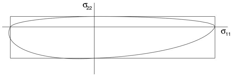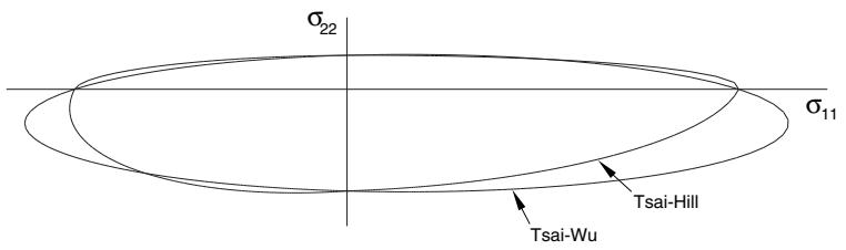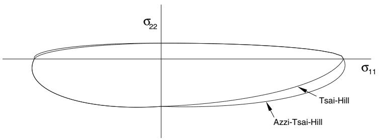# Stress-based failure measures—failure envelopes To illustrate the four stress-based failure measures, Figure 22.2.3–1, Figure 22.2.3–2, and Figure 22.2.3–3 show each failure envelope (i.e., $I _ { F } = 1 . 0 )$ in $\left( \sigma _ { 1 1 } - \sigma _ { 2 2 } \right)$ stress space compared to the Tsai-Hill envelope for a given value of in-plane shear stress. In each case the Tsai-Hill surface is the piecewise continuous elliptical surface with each quadrant of the surface defined by an ellipse centered at the origin. The parallelogram in Figure 22.2.3–1 defines the maximum stress surface. In Figure 22.2.3–2 the Tsai-Wu surface appears as the ellipse. In Figure 22.2.3–3 the Azzi-Tsai-Hill surface differs from the Tsai-Hill surface only in the second and fourth quadrants, where it is the outside bounding surface (i.e., further from the origin). Since all of the failure theories are calibrated by tensile and compressive failure under uniaxial stress, they all give the same values on the stress axes. 

text_image

σ₂₂ σ₁₁

Figure 22.2.3–1 Tsai-Hill versus maximum stress failure envelope $( I _ { F } = 1 . 0 )$ . 

text_image

σ₂₂ σ₁₁ Tsai-Hill Tsai-Wu

Figure 22.2.3–2 Tsai-Hill versus Tsai-Wu failure envelope $( I _ { F } = 1 . 0 , F _ { 1 2 } = 0 . 0 )$ . 

text_image

σ₂₂ σ₁₁ Tsai-Hill Azzi-Tsai-Hill

Figure 22.2.3–3 Tsai-Hill versus Azzi-Tsai-Hill failure envelope $( I _ { F } = 1 . 0 )$ . # Strain-based failure theory The input data for the strain-based theory are tensile and compressive strain limits, $X _ { \varepsilon _ { t } }$ and $X _ { \varepsilon _ { c } } ,$ in the 1-direction; tensile and compressive strain limits, $Y _ { \varepsilon _ { t } }$ and $Y _ { \varepsilon _ { c } }$ , in the 2-direction; and shear strain limit, $S _ { \varepsilon } ,$ , in the X–Y plane. Input File Usage: \*FAIL STRAIN Abaqus/CAE Usage: Property module: material editor: Mechanical→Elasticity→Elastic: Suboptions→Fail Strain # Maximum strain theory $\mathrm { I f } \varepsilon _ { 1 1 } > 0 , X _ { \varepsilon } = X _ { \varepsilon _ { t } }$ ; otherwise, $X _ { \varepsilon } = X _ { \varepsilon _ { c } . } \mathrm { I f } \varepsilon _ { 2 2 } > 0 , Y _ { \varepsilon } = Y _ { \varepsilon _ { t } }$ ; otherwise, $Y _ { \varepsilon } = Y _ { \varepsilon _ { c } }$ . The maximum strain failure criterion requires that $$ I _ {F} = \max \left(\frac {\varepsilon_ {1 1}}{X _ {\varepsilon}}, \frac {\varepsilon_ {2 2}}{Y _ {\varepsilon}}, \left| \frac {\varepsilon_ {1 2}}{S _ {\varepsilon}} \right|\right) < 1. 0. $$