# RETRACTOR Connection type RETRACTOR joins the position of two nodes and provides a FLOW-CONVERTER constraint between the material flow degree of freedom (10) at the second node and the rotational degrees of freedom at the first node of the connector. This connection type can be used to model retractor and pretensioner devices in automotive seat belts (see “Seat belt analysis of a simplified crash dummy,” Section 3.3.1 of the Abaqus Example Problems Guide) or cable drums in winch-like devices. RETRACTOR connections cannot be used in two-dimensional and axisymmetric analyses in Abaqus/Explicit. 

text_image

axle or drum belt or cable wrapped belt or cable Lw e₃ᵃ a, b e₃ᵃ e₁ᵃ a, b e₂ᵃ

Figure 31.1.5–24 Connection type RETRACTOR. # Description Connection type RETRACTOR imposes kinematic constraints and uses local orientation definitions equivalent to combining connection types JOIN and FLOW-CONVERTER. # Summary

RETRACTOR
Basic, assembled, or complex:	Assembled
Kinematic constraints:	JOIN + FLOW-CONVERTER
Constraint force output:	$f_1, f_2, f_3, m_3$
Available components:	None
Kinetic force output:	None
Orientation at $a$ :	Required
Orientation at $b$ :	Ignored

RETRACTOR

Connector stops:	None
Constitutive reference lengths:	None
Predefined friction parameters:	None
Contact force for predefined friction:	None

# REVOLUTE Connection type REVOLUTE provides a connection between two nodes where the rotations are constrained about two local directions and free about a shared axis. The shared axis of rotation is the connector local 1-direction. Connection type REVOLUTE cannot be used in two-dimensional or axisymmetric analysis. Connection type REVOLUTE models the rotational part of a HINGE or CYLINDRICAL joint. 

text_image

e₁ᵃ e₁ᵇ e₁ᵃ e₁ᵇ e₁ᵃ e₁ᵇ e₁ᵃ e₁ᵇ e₁ᵃ e₁ᵇ e₁ᵃ e₁ᵇ e₁ᵃ e₁ᵇ e₁ᵃ e₁ᵇ e₁ᵃ e₁ᵇ e₁ᵃ e₁ᵇ e₁ᵃ e₁ᵇ e₁ᵃ e₁ᵇ e₁ᵃ e₁ᵇ e₁ᵃ

Figure 31.1.5–25 Connection type REVOLUTE. # Description A REVOLUTE connection constrains two rotational components of relative motion between two nodes and allows one free rotational component. The two kinematic constraints imposed by the REVOLUTE connection are $$ \mathbf {e} _ {1} ^ {a} \cdot \mathbf {e} _ {2} ^ {b} = 0 \quad \text {and} \quad \mathbf {e} _ {1} ^ {a} \cdot \mathbf {e} _ {3} ^ {b} = 0 , $$ which are equivalent to the requirement that ${ \bf e } _ { 1 } ^ { a } = { \bf e } _ { 1 } ^ { b }$ . Alternatively, the REVOLUTE constraint is equivalent to setting the second and third Cardan angles to zero in a CARDAN connection. If the shared axes ${ \bf e } _ { 1 } ^ { a }$ and $\mathbf { e } _ { 1 } ^ { b }$ do not align initially, the REVOLUTE constraint will hold the second and third Cardan angles fixed at their initial values. The constraint moment in the REVOLUTE connection is $$ \bar {\bf m} = m _ {2} {\bf e} _ {2} ^ {a} + m _ {3} {\bf e} _ {3} ^ {a}. $$ Node b can rotate about the shared local direction ${ \bf e } _ { 1 } ^ { a } = { \bf e } _ { 1 } ^ { b }$ . The relative angular position of the local directions at node b relative to a is $$ \alpha = - \tan^ {- 1} \left(\frac {\mathbf {e} _ {2} ^ {a} \cdot \mathbf {e} _ {3} ^ {b}}{\mathbf {e} _ {3} ^ {a} \cdot \mathbf {e} _ {3} ^ {b}}\right), $$ where is the first Cardan angle measuring a counterclockwise rotation about the ${ \bf e } _ { 1 } ^ { a }$ -direction of $\mathbf { { \dot { e } } } _ { 2 } ^ { a }$ to $\mathbf { e } _ { 2 } ^ { b }$ . The available component of relative motion, $u r _ { 1 }$ , measures the change in angular position and is defined as $$ u r _ {1} = \alpha - \alpha_ {0} + n \pi , $$ where $\alpha _ { 0 }$ is the initial angular position and n is an integer accounting for multiple rotations about the shared axis. The connector constitutive rotation is $$ u r _ {1} ^ {m a t} = \alpha - \theta_ {1} ^ {r e f} + n \pi . $$ The kinetic moment in the REVOLUTE connection is $$ \mathbf {m} _ {r e v o l u t e} = m _ {1} \mathbf {e} _ {1} ^ {a}. $$ # Friction When used by itself, there is no predefined Coulomb-like friction in the REVOLUTE connection. However, when the REVOLUTE connection is used in combination with a JOIN, SLIDE-PLANE, or SLOT connection, the predefined friction is the same as the HINGE, PLANAR, and CYLINDRICAL connections, respectively. # Summary REVOLUTE

Basic, assembled, or complex:	Basic
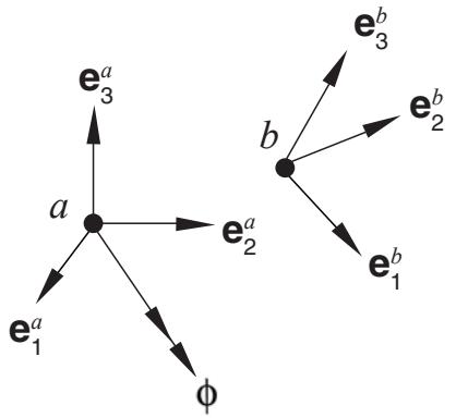
Kinematic constraints:	$\mathbf{e}_{1}^{a} \cdot \mathbf{e}_{2}^{b} = 0, \mathbf{e}_{1}^{a} \cdot \mathbf{e}_{3}^{b} = 0$
Constraint moment output:	$m_{2}, m_{3}$
Available components:	$ur_{1}$
Kinetic moment output:	$m_{1}$
Orientation at a:	Required
Orientation at b:	Optional
Connector stops:	$\theta_{1}^{min} \leq \alpha \leq \theta_{1}^{max}$
Constitutive reference angles:	$\theta_{1}^{ref}$
Predefined friction parameters:	None
Contact moment for predefined friction:	None

# ROTATION Connection type ROTATION provides a rotational connection between two nodes where the relative rotation between the nodes is parameterized by the rotation vector. In two-dimensional and axisymmetric analyses, the ROTATION connection type involves a single (scalar) relative rotation component. Although available components of relative motion exist for the ROTATION connection type in three-dimensional analysis, the finite rotation parameterization of the connection is not necessarily well-suited for defining connector behavior. If a finite, three-dimensional ROTATION connection with connector behavior is desired, either the CARDAN or EULER connection type typically is more appropriate. When connection type ROTATION is used in a connector element connected to ground at the element’s first node, the rotational components relative to the orientation at ground are identical to the Abaqus convention for nodal rotation degrees of freedom. Hence, connection type ROTATION can be used in conjunction with prescribed connector motion (see “Connector actuation,” Section 31.1.3) to specify finite rotation boundary conditions in local coordinate directions using the Abaqus convention for finite rotation boundary conditions. 

flowchart

```mermaid graph TD A["φ"] --> B["1"] A --> C["2"] A --> D["3"] B --> E["1"] B --> F["2"] B --> G["3"] C --> H["1"] C --> I["2"] C --> J["3"] E --> K["1"] E --> L["2"] E --> M["3"] F --> N["1"] F --> O["2"] F --> P["3"] G --> Q["1"] G --> R["2"] G --> S["3"] H --> T["1"] H --> U["2"] H --> V["3"] I --> W["1"] I --> X["2"] I --> Y["3"] J --> Z["1"] J --> AA["2"] J --> AB["3"] ```

Figure 31.1.5–26 Connection type ROTATION. # Description The rotation connection does not impose kinematic constraints. The rotation connection is a finite rotation connection where the local directions at node b are parameterized relative to the local directions at node a by the rotation vector. Let be the rotation vector that positions local directions $\{ \mathbf { e } _ { 1 } ^ { b } , \mathbf { e } _ { 2 } ^ { b } , \mathbf { e } _ { 3 } ^ { b } \}$ relative to $\{ \mathbf { e } _ { 1 } ^ { a } , \mathbf { e } _ { 2 } ^ { a } , \mathbf { e } _ { 3 } ^ { a } \}$ ; that is, $$ \mathbf {e} _ {i} ^ {b} = \exp \left[ \hat {\phi} \right] \cdot \mathbf {e} _ {i} ^ {a} $$ for all $i = { 1 , 2 , 3 }$ , where $\hat { \phi }$ is the skew-symmetric matrix with axial vector $\phi .$ . See “Rotation variables,” Section 1.3.1 of the Abaqus Theory Guide, for a discussion of finite rotations. The available components of relative motion in the ROTATION connection are the change in the rotation vector components positioning the local directions at node $\pmb { b }$ relative to the local directions at node a. Therefore, $$ u r _ {i} = \phi_ {i} - (\phi_ {0}) _ {i} + 2 n \pi \frac {\phi_ {i}}{\| \phi \|}, $$ where $\phi _ { 0 }$ is the initial rotation vector, $n \geq 0$ is an integer accounting for rotations with magnitude greater than $2 \pi$ , all vector components are components relative to the local directions ${ \bf e } _ { i } ^ { a }$ , and $i = { 1 , 2 , 3 }$ . The connector constitutive rotations are $$ u r _ {i} ^ {m a t} = \phi_ {i} - \theta_ {i} ^ {r e f} + 2 n \pi \frac {\phi_ {i}}{\| \phi \|}. $$ The kinetic moment in a rotation connection is $$ m _ {i} = \mathbf {m} _ {r o t a t i o n} \cdot \mathbf {e} _ {i} ^ {a}, i = 1, 2, 3. $$ In two-dimensional and axisymmetric analyses $u r _ { 1 } = u r _ { 2 } = 0$ and $m _ { 1 } = m _ { 2 } = 0$ . # Summary ROTATION

Basic, assembled, or complex:	Basic
Kinematic constraints:	None
Constraint moment output:	None
Available components:	$ur_{1}, ur_{2}, ur_{3}$
Kinetic moment output:	$m_{1}, m_{2}, m_{3}$
Orientation at a:	Optional
Orientation at b:	Optional
Connector stops:	$\theta_{i}^{min} \leq \phi_{i} \leq \theta_{i}^{max}$
Constitutive reference angles:	$\theta_{i}^{ref}$
Predefined friction parameters:	None
Contact force for predefined friction:	None

# ROTATION-ACCELEROMETER Connection type ROTATION-ACCELEROMETER provides a convenient way to measure the relative angular position, velocity, and acceleration of a body in a local coordinate system. These kinematic quantities are measured relative to the motion of node a and are reported in the coordinate system of node b. Each node of the connector can translate and rotate independently, although fixing the first of the two nodes to ground is more common. With the first node fixed, connection type ROTATION-ACCELEROMETER provides a convenient way to measure the local components of the angular velocity and angular acceleration in a coordinate system fixed to a moving body (for example, an accelerometer). Connection type ROTATION-ACCELEROMETER is available only in Abaqus/Explicit. It is the rotation counterpart to connection type ACCELEROMETER, which measures relative translational position, velocity, and acceleration. ROTATION-ACCELEROMETER connectors cannot be used in two-dimensional and axisymmetric analysis in Abaqus/Explicit. 

text_image

e₃ᵃ a e₂ᵃ e₁ᵃ φ e₃ᵇ b e₂ᵇ e₁ᵇ

Figure 31.1.5–27 Connection type ROTATION-ACCELEROMETER. # Description The ROTATION-ACCELEROMETER connection does not impose kinematic constraints. It defines three local directions at node a and three local directions at node b. The ROTATION-ACCELEROMETER connection’s formulation is similar to that for the ROTATION connection. The ROTATION-ACCELEROMETER connection measures the finite rotation that takes the local directions at node a into the local directions at node b and parameterizes that finite rotation by the rotation vector. Let be the rotation vector that positions local directions $\{ \mathbf { e } _ { 1 } ^ { b } , \mathbf { e } _ { 2 } ^ { b } , \mathbf { e } _ { 3 } ^ { b } \}$ relative to $\{ \mathbf { e } _ { 1 } ^ { a } , \mathbf { e } _ { 2 } ^ { a } , \mathbf { e } _ { 3 } ^ { a } \}$ ; that is, $$ \mathbf {e} _ {i} ^ {b} = \exp \left[ \hat {\phi} \right] \cdot \mathbf {e} _ {i} ^ {a} $$ for all $i = { 1 , 2 , 3 }$ , where $\hat { \phi }$ is the skew-symmetric matrix with axial vector . See “Rotation variables,” Section 1.3.1 of the Abaqus Theory Guide, for a discussion of finite rotations. The connection measures the change in the rotation vector components in the local directions rotating with the body at node b. The rotation vector components are calculated as $$ \phi_ {i} = \mathbf {e} _ {i} ^ {b} \cdot \phi . $$ There are no available components of relative motion for the ROTATION-ACCELEROMETER connection. The connector rotation is $$ u r _ {i} = \phi_ {i} - (\phi_ {0}) _ {i} + 2 n \pi \frac {\phi_ {i}}{| | \phi | |}, $$ where $\phi _ { 0 }$ is the initial rotation vector and $n \geq 0$ is an integer accounting for rotations with magnitude greater than . The ROTATION-ACCELEROMETER connection differs from the ROTATION connection in the way angular velocity and acceleration are calculated. The ROTATION-ACCELEROMETER connection measures velocity and acceleration from the nodes as $$ v r _ {i} = (\omega_ {b} - \omega_ {a}) \cdot \mathbf {e} _ {i} ^ {b} \quad \text {and} \quad a r _ {i} = (\alpha_ {b} - \alpha_ {a}) \cdot \mathbf {e} _ {i} ^ {b}, $$ where $\omega _ { a } , \omega _ { b } , \alpha _ { a }$ , and $\alpha _ { b }$ are the nodal angular velocities and accelerations at nodes a and b, respectively. In two-dimensional and axisymmetric analyses $u r _ { 1 } = u r _ { 2 } = 0$ . Summary

ROTATION-ACCELEROMETER
Basic, assembled, or complex:	Basic
Kinematic constraints:	None
Constraint force output:	None
Available components:	None
Kinetic force output:	None
Orientation at a:	Optional
Orientation at b:	Optional
Connector stops:	None
Constitutive reference lengths:	None
Predefined friction parameters:	None
Contact force for predefined friction:	None

# SLIDE-PLANE Connection type SLIDE-PLANE keeps node b on a plane defined by the orientation of node a and the initial position of node b. Connection type SLIDE-PLANE cannot be used in two-dimensional or axisymmetric analysis. The normal direction defining the plane at node a is ${ \bf e } _ { 1 } ^ { a }$ . Connection type SLIDE-PLANE models a point confined between parallel plates or a pin-in-slot connection where the pin is free to move normal to the plane of the slot. 

text_image

e₁ᵃ a e₂ᵃ e₃ᵃ X₀ b u₂ u₃

Figure 31.1.5–28 Connection type SLIDE-PLANE. # Description The SLIDE-PLANE connection constrains the position of node ${ \pmb b } , { \bf x } _ { b }$ , to remain on a plane defined by the local normal direction ${ \bf e } _ { 1 } ^ { a }$ . The normal direction distance from node a to the plane is constant: $$ x = \mathbf {e} _ {1} ^ {a} \cdot (\mathbf {x} _ {b} - \mathbf {x} _ {a}) = x _ {0}, $$ where $x _ { 0 }$ is the initial distance from node a to the plane. The constraint force in the SLIDE-PLANE connection is $$ \bar {\mathbf {f}} = f _ {1} \mathbf {e} _ {1} ^ {a}. $$ Node b can move in the plane defined by the normal of node a. The position of node b in the plane relative to node a is $$ y = \mathbf {e} _ {2} ^ {a} \cdot (\mathbf {x} _ {b} - \mathbf {x} _ {a}) \quad \mathrm{and} \quad z = \mathbf {e} _ {3} ^ {a} \cdot (\mathbf {x} _ {b} - \mathbf {x} _ {a}). $$ The two available components of relative motion, $u _ { 2 }$ and $u _ { 3 } .$ , are $$ u _ {2} = y - y _ {0} \quad \text { and } \quad u _ {3} = z - z _ {0} , $$ where $y _ { 0 }$ and $z _ { 0 }$ are the coordinates of the initial position of node $\pmb { b . }$ The connector constitutive displacements are $$ u _ {2} ^ {m a t} = y - l _ {2} ^ {r e f} \quad \mathrm{and} \quad u _ {3} ^ {m a t} = z - l _ {3} ^ {r e f}. $$ The kinetic force in the plane is $$ \mathbf {f} _ {s - p} = f _ {2} \mathbf {e} _ {2} ^ {a} + f _ {3} \mathbf {e} _ {3} ^ {a}. $$ # Friction Predefined Coulomb-like friction in the SLIDE-PLANE connection relates the kinematic constraint forces in the connector to the friction forces (CSFC) in the translations along the two local directions in the 2–3 plane. The frictional effect is formally written as $$ \Phi = \mathrm{P} (\mathbf {f}) - \mu \mathrm{F} _ {\mathrm{N}} \leq 0, $$ where the potential $\mathrm { P } ( \mathbf { f } )$ represents the magnitude of the frictional tangential tractions in the connector in a direction tangent to the 2–3 plane on which contact occurs, $\mathrm { F _ { N } }$ is the friction-producing normal force on the same plane, and $\mu$ is the friction coefficient. Frictional stick occurs if $\Phi < 0 ;$ and sliding occurs if $\Phi = 0$ , in which case the friction force is $\mu \mathrm { F _ { N } }$ . The normal force $\mathrm { F _ { N } }$ is the sum of a magnitude measure of friction-producing connector forces, $\mathrm { F } _ { \mathrm { C } } = g ( \mathbf { f } )$ , and a self-equilibrated internal contact force, $\mathrm { F _ { C } ^ { \mathrm { i n t } } }$ : $$ \mathrm {F_ {N}} = | \mathrm {F_ {C}} + \mathrm {F_ {C} ^ {int}} | = | g (\mathbf {f}) + \mathrm {F_ {C} ^ {int}} |. $$ The force magnitude $\operatorname { F c } = | f _ { 1 } |$ . The magnitude of the frictional tangential tractions, $\mathrm { P } ( \mathbf { f } )$ is computed using $$ \mathrm{P} (\mathbf {f}) = \sqrt {f _ {2} ^ {2} + f _ {3} ^ {2}}. $$ The predefined Coulomb-like friction is computed differently when the SLIDE-PLANE connection is used in combination with a REVOLUTE connection. See the description of the PLANAR connection for the predefined friction definition in this case.