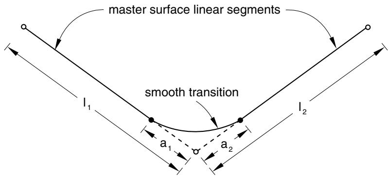
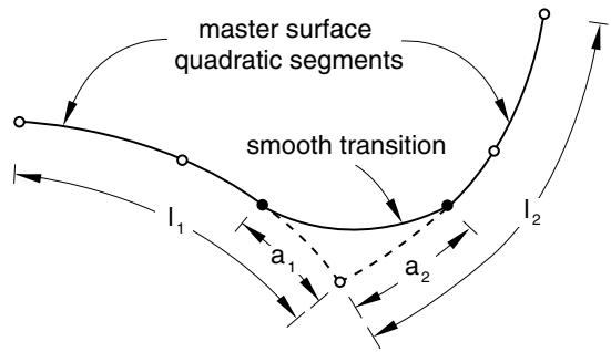
Smoothing deformable master surfaces and rigid surfaces defined with rigid elements For finite-sliding, node-to-surface contact simulations with planar or axisymmetric deformable master surfaces, Abaqus/Standard will smooth any discontinuous transitions between two first-order element faces with parabolic curves. Discontinuous transitions between two second-order element faces are smoothed with cubic curves connecting two points located on the element’s faces. This smoothing is shown in Figure 38.1.1–7 for first-order elements (linear segments) and in Figure 38.1.1–8 for second-order elements (parabolic segments). For finite-sliding, node-to-surface simulations with three-dimensional deformable master surfaces and rigid master surfaces using rigid elements, Abaqus/Standard will smooth any discontinuous surface normal transitions between the master surface facets. 

text_image

master surface linear segments smooth transition l₁ a₁ a₂ l₂

Figure 38.1.1–7 Smoothing between linear segments. 

text_image

master surface quadratic segments smooth transition I₁ a₁ a₂ I₂

Figure 38.1.1–8 Smoothing between quadratic segments. You can control the degree of smoothing of the master surface in node-to-surface contact simulations or in analyses using slide lines and contact elements by specifying a fraction $f .$ The default value of f is 0.2. For planar or axisymmetric deformable master surfaces, $f = a _ { 1 } / \ell _ { 1 } = a _ { 2 } / \ell _ { 2 }$ , where $\ell _ { 1 }$ and $\ell _ { 2 }$ are the lengths of the element facets that join at the surface node and $f \mathrm { ~ < ~ } 0 . 5$ (see Figure 38.1.1–7 and Figure 38.1.1–8). Abaqus/Standard will construct either a parabolic or a cubic segment between two points at distances $a _ { 1 }$ and $a _ { 2 }$ from the node at which the discontinuity exists; this smoothed segment will be used in the contact calculations. Thus, the contact surface will differ from the faceted element geometry. Smoothing affects only segments where the normal to the deformable master surface is discontinuous at the node joining two elements: it does not affect the two segments adjacent to the midside nodes on second-order element faces. For three-dimensional, element-based master surfaces, f is defined as a fraction of the dimension of a facet as shown in Figure 38.1.1–9. The normal vector of a point within the region bounded by the dashed lines is computed to be normal to the facet. Outside this region the normal is smoothed with respect to the adjacent facets, using a generalization of the two-dimensional approach shown in Figure 38.1.1–7 and Figure 38.1.1–8. The physical geometry of a three-dimensional facet is not smoothed; only the surface normal definitions associated with the facet are affected by the smoothing operation. The implementation of the normal-direction smoothing algorithm is slightly different for surfaces based on rigid type elements (see “Rigid elements,” Section 30.3.1) than other element types. This difference typically has minimal effect on the convergence behavior or solution results; however, for example, different solution behavior may occasionally be observed between otherwise identical analyses in which a rigid body is modeled with R3D4 elements in one case and S4R elements assigned to a rigid body in another case. 

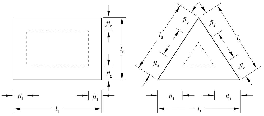
text_image

fl₂ l₂ fl₂ fl₃ fl₂ l₃ fl₃ fl₂ fl₁ l₁ fl₁ l₁ fl₁

Figure 38.1.1–9 Smoothing of a three-dimensional master surface. # Input File Usage: Use the following option for node-to-surface contact simulations: \*CONTACT PAIR, INTERACTION=interaction\_property\_name, SMOOTH=f Use the following option when using slide lines and contact elements: \*SLIDE LINE, ELSET=name, SMOOTH=f # Abaqus/CAE Usage: Interaction module: Interaction→Create: Surface-to-surface contact (Standard) or Self-contact (Standard): Degree of smoothing for master surface: f Smoothing a deformable master surface along symmetry edges When a two-dimensional or axisymmetric deformable master surface ends at a symmetry plane and node-to-surface discretization is used, Abaqus/Standard will smooth and calculate the proper surface normals and tangent planes of the end segment if the boundary condition at the symmetry end is specified with the symmetry “type” boundary XSYMM or YSYMM. This smoothing procedure is accomplished by reflecting the end segment about the symmetry plane and constructing either a parabolic or a cubic segment between the end segment and the reflected segment. Thus, the contact surface may differ from the faceted element geometry near the end. Abaqus/Standard will automatically adjust the surface normal and tangent planes at of an axisymmetric master surface regardless of whether a symmetry boundary condition is defined. The finite-sliding, surface-to-surface formulation has no special treatment for surfaces ending at a symmetry plane. See “Modifying the master surface normals” in “Contact formulations in Abaqus/Standard,” Section 38.1.1, for a discussion of how the small-sliding, node-tosurface formulation treats master surfaces ending at a symmetry plane. See “Small-sliding, surface-tosurface contact” in “Contact formulations in Abaqus/Standard,” Section 38.1.1, for a discussion of how the small-sliding, node-to-surface formulation treats slave surfaces ending at a symmetry plane. Overriding the default smoothing behavior for finite-sliding, node-to-surface contact To model a master surface with corners in two dimensions (fold lines in three dimensions), break the surface into multiple surfaces. This technique prevents Abaqus/Standard from smoothing out the corners or fold lines and allows Abaqus/Standard to introduce constraints associated with each surface if a slave node is in contact with an interior corner or fold in the master surface. To accurately model the master surface with a corner shown in Figure 38.1.1–10, you must define two contact pairs: the first contact pair has ASURF as the slave surface and BSURFA as the master surface; the second contact pair has ASURF as the slave surface and BSURFB as the master surface. # Finite sliding in a geometrically linear analysis Finite-sliding simulations usually include nonlinear geometric effects because such simulations generally involve large deformations and large rotations. However, it is also possible to use the finite-sliding tracking approach in a geometrically linear analysis (see “Geometric nonlinearity” in “General and linear perturbation procedures,” Section 6.1.3). The load transfer paths between the surfaces and the contact direction are updated in finite-sliding, geometrically linear analyses. This capability is useful for analyzing finite sliding between two stiff bodies that do not undergo large rotations. # Unsymmetric terms in finite-sliding contact simulations Normal contact constraints due to node-to-surface discretization produce unsymmetric terms in the system of equations when three-dimensional faceted surfaces come in contact. These terms have a 

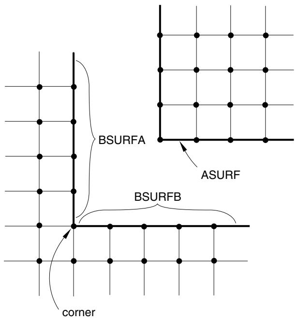
text_image

BSURFA ASURF BSURFB corner

Figure 38.1.1–10 Master surface with a corner. strong effect on the convergence rate in regions on the master surfaces with large differences in surface normals between facets. Normal contact constraints due to surface-to-surface discretization produce unsymmetric terms in both two- and three-dimensional cases. These terms have a strong effect on the convergence rate in regions where the master and slave surfaces are not parallel to each other. In both cases you should use the unsymmetric solution scheme for the step to improve the convergence rate of the simulation (see “Matrix storage and solution scheme in Abaqus/Standard” in “Defining an analysis,” Section 6.1.2). Contact simulations that involve strong frictional effects can also produce unsymmetric terms. See “Unsymmetric terms in the system of equations” in “Frictional behavior,” Section 37.1.5, for details. # Using the small-sliding tracking approach For a large class of contact problems the general tracking of the finite-sliding approach is unnecessary, even though geometric nonlinearity may need to be considered. Abaqus/Standard provides a smallsliding tracking approach for such problems. For geometrically nonlinear analyses this formulation assumes that the surfaces may undergo arbitrarily large rotations but that a slave node will interact with the same local area of the master surface throughout the analysis. For geometrically linear analyses the small-sliding approach reduces to an infinitesimal-sliding and rotation approach, in which it is assumed that both the relative motion of the surfaces and the absolute motion of the contacting bodies are small. 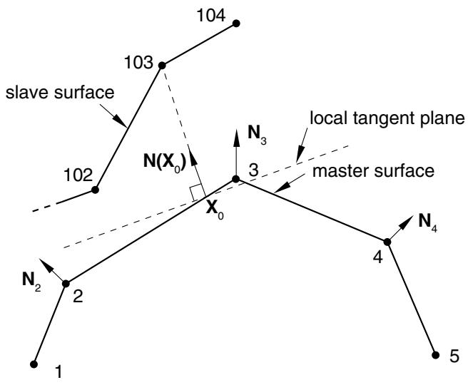Abaqus/Standard attempts to associate a planar approximation of the master surface with each slave node of a small-sliding contact pair. Contact interactions are considered between a given slave node (or region nearby a given slave node for the surface-to-surface formulation) and the associated local tangent plane. An example for the small-sliding, node-to-surface formulation is shown in Figure 38.1.1–11 (for example, the slave node is typically constrained not to penetrate this local tangent plane). Each local tangent plane, which is a line in two dimensions, is defined by an anchor point, $\mathbf { X } _ { 0 } .$ , on the master surface and an orientation vector at the anchor point (see Figure 38.1.1–11). 

text_image

104 103 slave surface 102 N(X₀) N₃ local tangent plane master surface X₀ 3 N₂ 2 4 N₄ 1 5

Figure 38.1.1–11 Definition of the anchor point and local tangent plane used by the small-sliding, node-to-surface formulation for node 103. The algorithm used to define anchor points is described below. If an anchor point cannot be determined for a particular slave node, no contact constraint will be enforced for that slave node. Having a local tangent plane for each slave node means that for the small-sliding tracking approach Abaqus/Standard does not have to monitor slave nodes for possible contact along the entire master surface. Therefore, small-sliding contact is generally less expensive computationally than finite-sliding contact. The cost savings are often most dramatic in three-dimensional contact problems. # Small-sliding, node-to-surface contact For node-to-surface contact Abaqus/Standard chooses the anchor point of a slave node’s local tangent plane such that the vector from the anchor point to the slave node coincides with a smoothly varying normal vector on the master surface. The anchor point is chosen before the analysis starts using the initial configuration of the model. # Smoothly varying master surface normals The algorithm requires that the master surface have a smoothly varying normal vector $\mathbf { N } ( \mathbf { x } )$ , where is any point on the master surface. The first step in defining $\mathbf { N } ( \mathbf { x } )$ is to construct the unit normal vectors at each node of the master surface. Abaqus/Standard forms these nodal normals by averaging the normals of the element faces making up the master surface; only the element faces in the surface definition will contribute to the nodal normals and, thus, to $\mathbf { N } ( \mathbf { x } )$ . Abaqus/Standard uses the initial nodal coordinates to compute these normals. Figure 38.1.1–11 shows the nodal unit normals for a master surface, the anchor point $\mathbf { X } _ { 0 } ,$ , and the local tangent plane associated with slave node 103. Abaqus/Standard uses the nodal unit normals $\mathbf { N _ { 2 } }$ and $\mathbf { N _ { 3 } }$ , along with the shape functions of the element containing the two nodes, to construct $\mathbf { N } ( \mathbf { x } )$ on the 2–3 element face. Abaqus/Standard chooses the anchor point $\mathbf { X } _ { 0 }$ of the local tangent plane for node 103 so that $\bf N ( X _ { 0 } )$ passes through node 103. $\bf ( X _ { 0 } )$ is the contact direction for slave node 103 and defines the orientation of the local tangent plane. In this example, as in many cases, the local tangent plane is only an approximation of the actual mesh geometry. 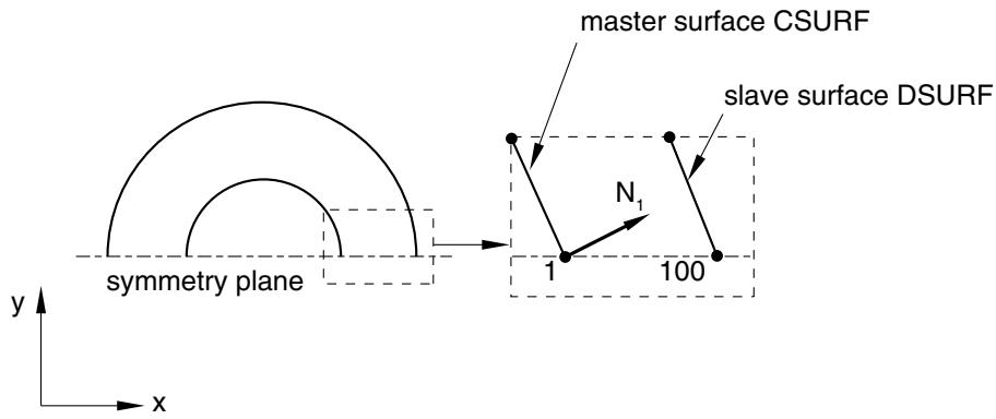# Modifying the master surface normals Defining user-specified nodal normals on the master surface (see “Normal definitions at nodes,” Section 2.1.4) will improve the local tangent planes calculated for the small-sliding, node-to-surface formulation in some cases. For example, a default nodal normal corresponding to an average normal among adjacent facets can cause significant deviation from the true surface normal direction at perimeter nodes, as shown in Figure 38.1.1–12. The nodal normal $\mathbf { N _ { 1 } }$ does not point along the symmetry plane, which means that slave node 100 will never intersect the master surface. In a small-sliding problem if a slave node fails to intersect the master surface at the start of the analysis, it will be free to penetrate the master surface because no local tangent plane will be formed. 

text_image

master surface CSURF slave surface DSURF N₁ 1 100 symmetry plane y x

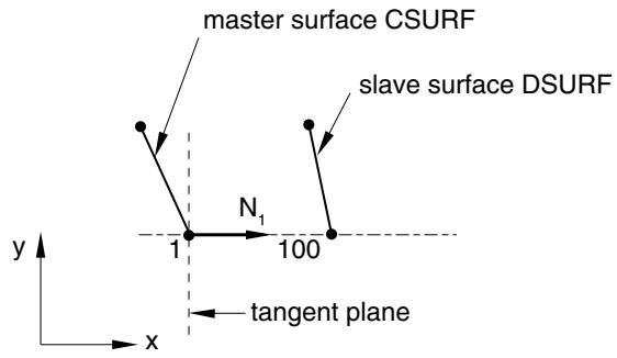
Figure 38.1.1–12 Master surface normal at node 1 in a small-sliding model of concentric cylinders. With the default $\mathbf { N _ { 1 } }$ slave node 100 will never contact CSURF. Defining a user-specified normal (1.00E+00, 0.00E+00, 0.00E+00) at node 1 on the master surface CSURF will correct the problem, as shown in Figure 38.1.1–13. This method allows slave node 100 to see the master surface, and the correct contact normal direction will be used. Master surface normals at perimeter nodes are adjusted automatically to lie along the symmetry plane if boundary conditions are specified at these nodes in symmetry “type” format (XSYMM, YSYMM, or ZSYMM—see “Boundary conditions in Abaqus/Standard and Abaqus/Explicit,” Section 34.3.1). 

text_image

master surface CSURF slave surface DSURF N₁ 1 100 y x tangent plane

Figure 38.1.1–13 The modified master surface normal at node 1 of CSURF now allows slave node 100 to contact CSURF. # Small-sliding, surface-to-surface contact A key difference with the surface-to-surface approach is that more than one slave node is involved in each contact constraint (except when the slave surface is based on gasket elements, as discussed below). This is related to the fact that the surface-to-surface formulation enforces contact conditions in an average sense over regions nearby slave nodes rather than only at individual slave nodes (see “Surfaceto-surface contact discretization” above). The small-sliding, surface-to-surface contact formulation is a limit case of the finite-sliding, surface-to-surface formulation, using a planar approximation of the master surface per averaging region of the slave surface. The constraint participation factors for the slave nodes remain constant for small-sliding contact. The effective center-of-action on the slave surface per contact constraint may differ slightly from the location of the predominant slave node associated with the constraint. A special version of the small-sliding, surface-to-surface formulation is used if the slave surface is based on gasket elements to avoid a tendency to trigger unstable deformation modes in the gasket elements. This special formulation has only one slave node per contact constraint and preserves the accuracy advantages of the surface-to-surface formulation, but it is not well-suited for extension to finite-sliding and is otherwise not as generally applicable as the regular small-sliding, surface-to-surface formulation. (The finite-sliding, surface-to-surface formulation always uses multiple slave nodes per constraint and is not recommended for contact involving gasket elements.) The small-sliding, surface-to-surface contact formulation determines master anchor points and normal directions in a manner similar to that used by the small-sliding, node-to-surface contact formulation; however, there are some differences. For the surface-to-surface approach the anchor point approximately corresponds to the center of the zone on the master surface where the averaging region of the slave projects onto the master surface. This projection occurs along the slave surface normal direction. This method does not make use of smoothed master surface nodal normals. The anchor point location typically does not depend significantly on whether node-to-surface or surface-to-surface discretization is used, unless the surfaces are significantly separated and non-parallel in the initial configuration (in which case small-sliding contact may not be appropriate). Abaqus/Standard automatically reverts to the node-to-surface approach for individual small-sliding contact constraints in the following circumstances, even if you have specified use of the surface-tosurface approach: • if the slave surface is a node-based surface; • if the projection along the slave surface normal direction does not intersect the master surface (but an anchor point can be found using the interpolated master surface normal direction algorithm discussed above for the small-sliding, node-to-surface formulation); or • if single-sided slave and master surfaces have surface normals in approximately the same direction. For constraints based on surface-to-surface discretization it is not necessary that the constraint associated with a node on a symmetry plane is parallel to the symmetry plane. Hence, there is usually no need to specify specific normal directions. As in the case of node-to-surface contact, the contact direction points from the anchor point to the slave node, and the tangent plane is normal to this direction. The contact normal for the small-sliding, surface-to-surface formulation is adjusted automatically to lie along the symmetry plane for each slave node that has a boundary condition specified in symmetry “type” format (XSYMM, YSYMM, or ZSYMM—see “Boundary conditions in Abaqus/Standard and Abaqus/Explicit,” Section 34.3.1). # Orientation of local tangent planes The local tangent plane is by definition orthogonal to the contact direction. You can override the default contact direction to specify a direction with a spatially varying clearance or overclosure definition (see “Specifying the surface normal for the contact calculations” in “Adjusting initial surface positions and specifying initial clearances in Abaqus/Standard contact pairs,” Section 36.3.5). Once the contact direction is defined, the orientation of the local tangent plane with respect to the master surface facet remains fixed. Because small-sliding contact considers nonlinear geometric effects, Abaqus/Standard continuously updates the orientation of the local tangent plane to account for the rotation and, assuming that the master surface is deformable, the deformation of the master surface. The position of the anchor point relative to the surrounding nodes on the master surface facet does not change as the master surface deforms. # Load transfer In a small-sliding analysis each constraint can transfer load only to a limited number of nodes on the master surface. These nodes on the master surface are chosen based on their initial proximity to the anchor point. The magnitude of load transferred to each master surface node is based on proximity in the current, deformed configuration to the center-of-action on the slave surface (which corresponds to a slave node for the node-to-surface formulation). For example, in Figure 38.1.1–11 node 103 transmits load to both nodes 2 and 3 on the master surface if node-to-surface discretization is used (if surface-to-surface discretization is used, load may be transmitted to additional nearby master nodes). Thus, if node 103 contacts the local tangent plane, a larger share of the force would be transmitted to the master surface node, 2 or 3, closer to the slave node. When the anchor point $\mathbf { X } _ { 0 }$ corresponds to a node on the master surface, as is the case with slave node 104 and master surface node 3 in Figure 38.1.1–11, the transmitted load for node-to-surface contact is shared by the node at $\mathbf { X } _ { 0 }$ and all of the master surface nodes that share an adjacent surface facet with that node (additional master nodes may take part in the load transfer for surface-to-surface contact). In Figure 38.1.1–11 the three master surface nodes sharing the force transmitted by slave node 104 are nodes 2, 3, and 4. 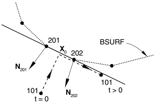As the center-of-action on the slave surface for a constraint slides along its local tangent plane, Abaqus/Standard updates the distribution among the master surface nodes. However, no additional master surface nodes are ever added to the original list of nodes associated with a given small-sliding constraint. The constraint will continue to transmit load to the original list of master surface nodes, regardless of the sliding distance. Figure 38.1.1–14 shows the potential problem that arises if small sliding is used but the relative tangential motion of the surfaces is not “small.” It shows the possible evolution of contact between slave node 101 in Figure 38.1.1–5 and its master surface BSURF. Using the unit normal vectors $\mathbf { N } _ { 2 0 1 }$ and $\mathbf { N } _ { 2 0 2 }$ , the anchor point $\mathbf { X } _ { 0 }$ is found for slave node 101; for the purposes of this example, assume that it lies at the midpoint of the 201–202 face. With this location of $\mathbf { X } _ { 0 }$ the local tangent plane for node 101 is parallel with the 201–202 face. The load transfer always occurs between node 101 and nodes 201 and 202, no matter how far node 101 slides along the local tangent plane. Therefore, if node 101 moves as shown in Figure 38.1.1–14, it will continue to transmit load to nodes 201 and 202 when, in fact, it really slid off the mesh forming the master surface BSURF. 

text_image

201 X₀ 202 BSURF N₂₀₁ 101 t = 0 N₂₀₂ 101 t > 0

Figure 38.1.1–14 Excessive sliding in a small-sliding contact analysis. # What can be considered small sliding A contact pair in a small-sliding contact simulation should not grossly violate any of the assumptions or limitations outlined above. Adhere to the following guidelines: • Slave nodes should slide less than an element length from their corresponding anchor point and still be contacting their local tangent plane. If the master surface is highly curved, the slave nodes should slide only a fraction of an element length. The accumulated slip at a slave node (CSLIP) can provide a good estimate of how far a slave node has moved. • The local tangent planes formed by Abaqus/Standard should be a good approximation of the mesh geometry; if necessary, define a user-specified normal (“Normal definitions at nodes,” Section 2.1.4) to improve the smoothly varying master surface normal, . • The rotation and deformation of the master surface should not cause the local tangent planes to become a poor representation of the master surface during the course of the analysis. # Choosing the master and slave surfaces in small-sliding problems The basic guidelines given in “Defining contact pairs in Abaqus/Standard,” Section 36.3.1, should still be followed in a small-sliding simulation—the slave surface should be the more refined surface or the surface on the more deformable body. However, in a small-sliding simulation more thought must be given when defining the master surface. With small-sliding contact each slave node views the master surface as a flat surface, which can be significantly different than the true shape of the surface, even in the local region near the anchor point. In some cases the local tangent planes provide a good local approximation to the master surface in the initial configuration, but deformation and rotation of the master surface can reorient the local tangent planes such that they become a poor representation of the master surface. Figure 38.1.1–15 shows an example where distortion of the master surface results in such a situation. This problem can be minimized to some extent by using a more refined mesh on the master surface, thus providing more element faces to control the motion of the tangent planes. Excessive mesh refinement should not be necessary since only small sliding should occur. # Infinitesimal sliding As was mentioned before, the small-sliding tracking approach reduces to an infinitesimal-sliding tracking approach for geometrically linear analyses. Infinitesimal sliding assumes that both the relative motions of the surfaces and the absolute motions of the model remain small. The orientations of the local tangent planes are not updated, and the load transfer paths and the weightings assigned to each master surface node remain constant during an infinitesimal-sliding simulation. As in the case of small sliding, you can choose between node-to-surface and surface-to-surface discretizations with the infinitesimal-sliding tracking approach. The same user interface applies, and the default is node-to-surface discretization. # Local tangent directions on a surface Local tangent directions on a contact surface are a reference orientation by which Abaqus calculates tangential behavior in a contact interaction. Abaqus/Standard calculates the initial orientation of the two local tangent directions by default. The local tangent directions rotate with the contact surface in a geometrically nonlinear analysis.