coefficient, $\kappa _ { p }$ , is defined as a function of concentration. # 2.14 Substructuring # 2.14.1 Substructuring and superelement analysis The basic substructuring idea is to consider a "substructure" (a part of the model) separately and eliminate all but the degrees of freedom needed to connect this part to the rest of the model so that the substructure appears in the model as a "superelement": a collection of finite elements whose response is defined by the stiffness (and mass) of these retained degrees of freedom denoted by the vector, $\{ u ^ { R } \}$ . In ABAQUS/Standard the response within a substructure, once it has been reduced to a superelement, is considered to be a linear perturbation about the state of the substructure at the time it is made into a superelement. Thus, the substructure is in equilibrium with stresses ${ \pmb \sigma } _ { 0 } .$ , displacements $\mathbf { u } _ { 0 } .$ , and other state variables $h _ { 0 }$ when it is made into a superelement. Then, whenever it responds as a superelement, the total value of a displacement or stress component at some point within the substructure is $$ u = u _ {0} + \left\lfloor L _ {u} ^ {R} \right\rfloor \{\Delta u ^ {R} \} $$ $$ \sigma = \sigma_ {0} + \left\lfloor L _ {\sigma} ^ {R} \right\rfloor \{\Delta u ^ {R} \}, $$ where $\lfloor L _ { u } ^ { R } ( { \bf x } ) \rfloor$ and $\lfloor L _ { \sigma } ^ { R } ( \mathbf { x } ) \rfloor$ are linear transformations between the retained degrees of freedom of the superelement and the component of displacement or stress under consideration. The substructure must be in a self-equilibriating state when it is made into a superelement (except for reaction forces at prescribed boundary conditions that are applied to internal degrees of freedom in the superelement). If the substructure has been loaded to a nonzero state with some of its retained degrees of freedom fixed, these fixities are released at the time the superelement is created, and any reaction forces at them converted into concentrated loads that are part of the preload state. This means that the contribution of the superelement to the overall equilibrium of the model is defined entirely by its linear response. Since the purpose of the substructuring technique is to have the substructure contribute terms only to the retained degrees of freedom, we need to define its external load vector $\{ \overline { { { P } } } ^ { R } \} _ { \ r { \ r } } ,$ formed from the nonzero \*SLOADs applied to the superelement, and its internal force vector, $\{ \overline { { I } } ^ { R } \}$ , as a sum of linear transformations of the retained variables $\{ \Delta u ^ { R } \}$ and their velocities and accelerations: $$ \{\overline {{I}} ^ {R} \} = [ \overline {{M}} ] \{\ddot {u} ^ {R} \} + [ \overline {{C}} ] \{\dot {u} ^ {R} \} + [ \overline {{K}} ] \{\Delta u ^ {R} \}. $$ We refer to $[ \overline { { M } } ]$ as the reduced mass matrix for the superelement, $[ \overline { { C } } ]$ as its reduced damping matrix, and $[ \overline { { K } } ]$ as its reduced stiffness. These "reduced" mass, damping, and stiffness matrices connect the retained degrees of freedom only. The reduced stiffness matrix is easily derived when only static response is considered. Since the response of a superelement is entirely linear, its contribution to the virtual work equation for the model of which it is a part is # Procedures $$ \delta W = \left\lfloor \delta u ^ {R} \quad \delta u ^ {E} \right\rfloor \left(\left\{ \begin{array}{l} \Delta P ^ {R} \\ \Delta P ^ {E} \end{array} \right\} - \left[ \begin{array}{l l} K ^ {R R} & K ^ {R E} \\ K ^ {E R} & K ^ {E E} \end{array} \right] \left\{ \begin{array}{l} \Delta u ^ {R} \\ \Delta u ^ {E} \end{array} \right\}\right), $$ where $\{ \Delta P ^ { R } \}$ and $\{ \Delta P ^ { E } \}$ are consistent nodal forces applied to the substructure during its loading as a superelement (they do not include the self-equilibriating preloading of the substructure), and $$ [ K ] = \left[ \begin{array}{c c} K ^ {R R} & K ^ {R E} \\ K ^ {E R} & K ^ {E E} \end{array} \right] $$ is its tangent stiffness matrix. Since the internal degrees of freedom in the superelement, $\{ u ^ { E } \}$ , appear only within the superelement, the equilibrium equations conjugate to $\{ \delta u ^ { E } \}$ in the contribution to the virtual work equation given above are complete within the superelement, so that $$ \{\Delta P ^ {E} \} - [ K ^ {E R} ] \{\Delta u ^ {R} \} - [ K ^ {E E} ] \{\Delta u ^ {E} \} = 0. $$ These equations can be rewritten to define $\Delta u ^ { E }$ as Equation 2.14.1-1 $$ \{\Delta u ^ {E} \} = [ K ^ {E E} ] ^ {- 1} \left(\{\Delta P ^ {E} \} - [ K ^ {E R} ] \{\Delta u ^ {R} \}\right). $$ The superelement's contribution to the static equilibrium equations is, therefore, $$ \delta W = \left\lfloor \delta u ^ {R} \right\rfloor \left(\left(\left\{\Delta P ^ {R} \right\} - [ K ^ {R E} ] [ K ^ {E E} ] ^ {- 1} \left\{\Delta P ^ {E} \right\}\right) - \left([ K ^ {R R} ] - [ K ^ {R E} ] [ K ^ {E E} ] ^ {- 1} [ K ^ {E R} ]\right) \left\{\Delta u ^ {R} \right\}\right). $$ Thus, for static analysis the superelement's reduced stiffness is $$ [ \overline {{K}} ] = [ K ^ {R R} ] - [ K ^ {R E} ] [ K ^ {E E} ] ^ {- 1} [ K ^ {E R} ], $$ and the contribution of the \*SLOADs applied to the superelement is the load vector $$ \{\overline {{P}} ^ {R} \} = \{\Delta P ^ {R} \} - [ K ^ {R E} ] [ K ^ {E E} ] ^ {- 1} \{\Delta P ^ {E} \}. $$ The static modes defined by Equation 2.14.1-1 may not be sufficient to define the dynamic response of the superelement accurately. The superelement's dynamic representation may be improved by retaining additional degrees of freedom not required to connect the superelement to the rest of the model; that is, some of the $u ^ { E }$ can be moved into $u ^ { R }$ . This technique is known as Guyan reduction. An additional, and generally more effective, technique is to augment the response within the superelement by including some generalized degrees of freedom, $q ^ { \alpha }$ , associated with natural modes of the substructure. The simplest such approach is to extract some natural modes from the substructure with all retained degrees of freedom constrained, so that Equation 2.14.1-1 is augmented to be # Procedures $$ \{\Delta u ^ {E} \} = [ K ^ {E E} ] ^ {- 1} \left(\{\Delta P ^ {E} \} - [ K ^ {E R} ] \{\Delta u ^ {R} \}\right) + \{\phi^ {E} \} ^ {\alpha} q ^ {\alpha}, $$ with the variation $$ \{\delta u ^ {E} \} = - [ K ^ {E E} ] ^ {- 1} [ K ^ {E R} ] \{\delta u ^ {R} \} + \{\phi^ {E} \} ^ {\alpha} \delta q ^ {\alpha} $$ and the time derivatives $$ \{\dot {u} ^ {E} \} = - [ K ^ {E E} ] ^ {- 1} [ K ^ {E R} ] \{\dot {u} ^ {R} \} + \{\phi^ {E} \} ^ {\alpha} \dot {q} ^ {\alpha} $$ $$ \{\ddot {u} ^ {E} \} = - [ K ^ {E E} ] ^ {- 1} [ K ^ {E R} ] \{\ddot {u} ^ {R} \} + \{\phi^ {E} \} ^ {\alpha} \ddot {q} ^ {\alpha}. $$ The $\{ \phi ^ { E } \} ^ { \alpha }$ are the eigenmodes of the substructure, obtained with all retained degrees of freedom constrained, and the $q ^ { \alpha }$ are the generalized displacements--the magnitudes of the response in these normal modes. The contribution of the superelement to the virtual work equation for the dynamic case is $$ \begin{array}{l} \left\{ \begin{array}{c c} \delta u ^ {R} & \delta u ^ {E} \end{array} \right\} \left(\left\{ \begin{array}{c} \Delta P ^ {R} \\ \Delta P ^ {E} \end{array} \right\} - \left[ \begin{array}{c c} M ^ {R R} & M ^ {R E} \\ M ^ {E R} & M ^ {E E} \end{array} \right] \left\{ \begin{array}{c} \ddot {u} ^ {R} \\ \ddot {u} ^ {E} \end{array} \right\} - \left[ \begin{array}{c c} C ^ {R R} & C ^ {R E} \\ C ^ {E R} & C ^ {E E} \end{array} \right] \left\{ \begin{array}{c} \dot {u} ^ {R} \\ \dot {u} ^ {E} \end{array} \right\} \right. \\ - \left[\begin{array}{c c}K ^ {R R}&K ^ {R E}\\K ^ {E R}&K ^ {E E}\end{array}\right]\left\{\begin{array}{c}\Delta u ^ {R}\\\Delta u ^ {E}\end{array}\right\}\left. \right), \\ \end{array} $$ where $$ [ M ] = \left[ \begin{array}{c c} M ^ {E E} & M ^ {E R} \\ M ^ {R E} & M ^ {R R} \end{array} \right] $$ is the substructure's mass matrix, $$ [ C ] = \left[ \begin{array}{c c} C ^ {E E} & C ^ {E R} \\ C ^ {R E} & C ^ {R R} \end{array} \right] $$ is its damping matrix, and $$ \{P \} = \left\{ \begin{array}{l} \Delta P ^ {R} \\ \Delta P ^ {E} \end{array} \right\} $$ is the nodal force vector in the superelement. With the assumed dynamic response within the superelement, the internal degrees of freedom in this contribution $( \Delta u ^ { E }$ and its time derivatives) can be transformed to the retained degrees of freedom and the normal mode amplitudes, reducing the system to $$ \left\lfloor \delta u ^ {R} \quad \delta q \right\rfloor \left([ T ] ^ {T} \left\{P \right\} - [ T ] ^ {T} [ M ] [ T ] \left\{ \begin{array}{c} \ddot {u} ^ {R} \\ \ddot {q} \end{array} \right\} - [ T ] ^ {T} [ C ] [ T ] \left\{ \begin{array}{c} \dot {u} ^ {R} \\ \dot {q} \end{array} \right\} - [ T ] ^ {T} [ K ] [ T ] \left\{ \begin{array}{c} \Delta u ^ {R} \\ \Delta q \end{array} \right\}\right), $$ where $$ [ T ] = \left[ \begin{array}{c c} [ I ] & [ 0 ] \\ - [ K ^ {E E} ] ^ {- 1} [ K ^ {E R} ] & [ \phi^ {E} ] \end{array} \right], $$ in which [ÁE ] is the matrix of eigenvectors, fqg is the vector of generalized degrees of freedom, [I] is a unit matrix, and [0] is a null matrix. # 2.15 Submodeling # 2.15.1 Submodeling analysis Submodeling is the technique of studying a local part of a model with a refined mesh, based on interpolation of the solution from an initial, global model onto the nodes on the appropriate parts of the boundary of the submodel. The method is most useful when it is necessary to obtain an accurate, detailed solution in the local region and the detailed modeling of that local region has negligible effect on the overall solution. The response at the boundary of the local region is defined by the solution for the global model and it, together with any loads applied to the local region, determines the solution in the submodel. The technique relies on the global model defining this submodel boundary response with sufficient accuracy. Submodeling can be applied quite generally in ABAQUS. With a few restrictions different element types can be used in the submodel compared to those used to model the corresponding region in the global model. Both the global model and the submodel can use solid elements, or they can both use shell elements. A special option is available to use a submodel consisting of solid elements with a global model consisting of shell elements. The material response defined for the submodel may also be different from that defined for the global model. Both the global model and the submodel can have nonlinear response and can be analyzed for any sequence of analysis procedures. The procedures do not have to be the same for both models. The submodel is run as a separate analysis. The only link between the submodel and the global model is the transfer of the time-dependent values of variables to the relevant boundary nodes (the "driven nodes") of the submodel. The only information in the global model available to the submodel analysis is the file output data written during the global model analysis. It contains, by default, the undeformed coordinates of all global model nodes and element information for all elements in the global model (see \`\`Results file output format,'' Section 5.1.2 of the ABAQUS/Standard User's Manual). The user must have requested nodal responses in the area where the submodel boundary is located. These responses are used to prescribe boundary conditions at the driven nodes in the submodel. For details of the options used in the submodeling technique, see \`\`Submodeling,'' Section 7.3.1 of the ABAQUS/Standard User's Manual. # Interpolation procedure and tolerance checking In the solid-to-solid case the positions of the submodel boundary nodes (the driven nodes) are determined with respect to the global model, and the appropriate element interpolation functions are used to obtain the values of the degrees of freedom at the driven nodes. An "exterior tolerance," which can be set on the \*SUBMODEL option, is used to check whether it is valid to extrapolate values from the global model. The extrapolation is valid if the distance between the driven nodes and the free surface of the global model falls within the specified tolerance. 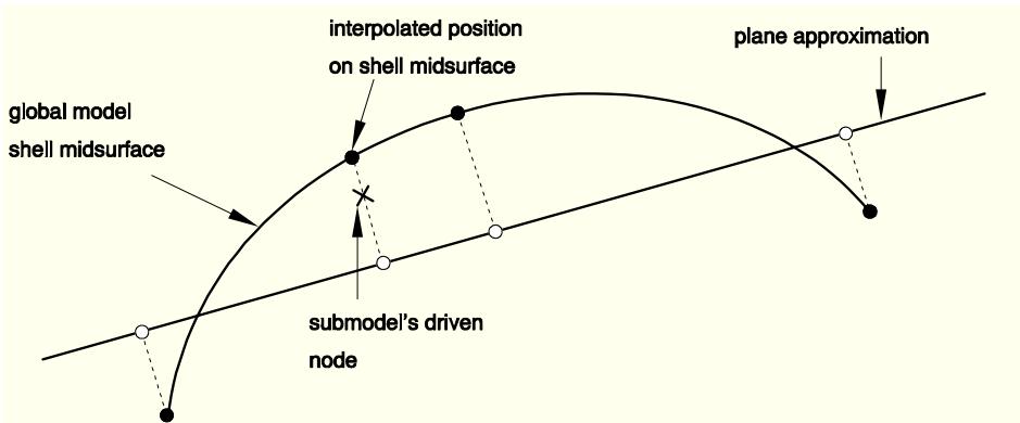A similar check is done along the global model boundaries for the shell-to-shell submodeling case. We also check whether the driven nodes of the submodel lie sufficiently close to the midsurface of the shell elements in the global model. To simplify the calculations, the closest point in the global model is approximated by measuring the distance in the direction normal to a flat approximation to each shell element in the global model, as shown in Figure 2.15.1-1. Figure 2.15.1-1 Flat surface approximation in shell-to-shell submodeling. 

flowchart

```mermaid graph TD A["global model shell midsurface"] --> B["interpolated position on shell midsurface"] B --> C["plane approximation"] C --> D["submodel's driven node"] D --> A ```

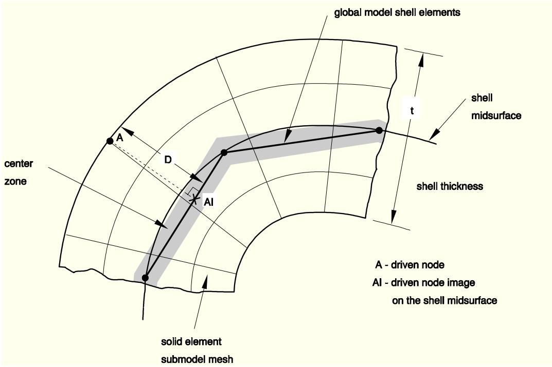
For the shell-to-solid case ABAQUS uses two kinds of tolerances to determine the relation between the submodel and the global model. First, the closest point on the shell midsurface of the global model is determined. This point will subsequently be referred to as the "image node" of the driven node. The exterior tolerance parameter is used to check if the image node lies within the domain of the global model. Then the distance between the driven node and its image is checked against half of the maximum shell thickness specified by the user (see Figure 2.15.1-2). Figure 2.15.1-2 Center zone in shell-to-solid submodeling. 

text_image

global model shell elements shell midsurface t shell thickness center zone A D AI A - driven node AI - driven node image on the shell midsurface solid element submodel mesh

If the node is within the half thickness plus the exterior tolerance, it is accepted. This check is only approximate if the global model has varying shell thickness, and in that case it will not protect the user in parts of the global model that have a small thickness compared to the maximum thickness specified on the \*SUBMODEL option. After the locations of the driven nodes (or image nodes for the shell-to-solid case) are determined, the prescribed values of the driven variables are interpolated from the values written to the file output for the global model. These must have been written with a sufficiently high frequency to obtain accurate values at the driven nodes. All components of displacements, temperatures, charges, and--for complex steady-state dynamic analysis--the phase angles as well as the amplitudes have to be written for the global model nodes from which the values for the driven nodes will be interpolated. For small global models responses will typically be written for all nodes. For large global models node sets can be created that contain the nodes in the regions around the submodel boundary. For solid-to-solid and shell-to-shell submodeling, the interpolated values of displacements, rotations, temperatures, etc. are applied directly to the driven nodes. For these nodes the user can specify the individual degrees of freedom that are driven. # Driven variables for shell-to-solid submodeling In the shell-to-solid case the driven degrees of freedom are chosen automatically, depending on the distance between the driven node and the midsurface of the shell. If the node lies within the center zone (specified on the \*BOUNDARY option), all displacement components are driven. If the node lies outside the center zone, only the displacement components parallel to the shell midsurface are driven. By default, the size of the center zone is taken as 10% of the maximum shell thickness. The procedure is described in detail below. The center zone should be large enough so that it contains at least one layer of nodes. If the transverse shear stresses at the submodel boundary are high and the submodel is highly refined in the thickness direction, this can result in high local stresses, since the shear force at the submodel boundary is only transferred at the driven nodes within the center zone. High transverse # Procedures shear stresses occur only in regions where bending moments vary rapidly, and it is better not to locate the submodel boundary in such regions. It is best to locate the submodel boundary in areas of low transverse shear stress in the global model. All displacement degrees of freedom are driven when the driven node lies within the center zone. For geometrically linear analysis these prescribed displacements are obtained from the displacements and rotations of the image node as Equation 2.15.1-1 $$ \mathbf {u} ^ {A} = \mathbf {u} ^ {A I} + \boldsymbol {\phi} ^ {A I} \times \mathbf {D}, $$ where $\mathbf { u } ^ { A }$ is the prescribed displacement of driven node $A , \mathbf { u } ^ { A I }$ and $\phi ^ { A I }$ are the interpolated displacement and rotation of the image node, and D is the vector connecting the image node to the driven node: $$ \mathbf {D} = \mathbf {X} ^ {A} - \mathbf {X} ^ {A I}. $$ For large-displacement analysis finite rotations must be taken into account. The finite rotation equivalent of Equation 2.15.1-1 is Equation 2.15.1-2 $$ \mathbf {u} ^ {A} = \mathbf {u} ^ {A I} + (\mathbf {C} - \mathbf {I}) \cdot \mathbf {D} = \mathbf {u} ^ {A I} + \mathbf {d} - \mathbf {D}, $$ where C is the rotation matrix as defined in \`\`Rotation variables,'' Section 1.3.1; I is the identity tensor; and d is the rotated vector connecting the image node to the driven node in the current configuration: $$ \mathbf {d} = \mathbf {C} \cdot \mathbf {D}. $$ For driven nodes outside the center zone only the displacement components parallel to the shell midsurface are driven. For the geometrically linear case this leads to the constraints Equation 2.15.1-3 $$ \mathbf {T} _ {1} \cdot \mathbf {u} ^ {A} = \mathbf {T} _ {1} \cdot (\mathbf {u} ^ {A I} + \boldsymbol {\phi} ^ {A I} \times \mathbf {D}), $$ $$ \mathbf {T} _ {2} \cdot \mathbf {u} ^ {A} = \mathbf {T} _ {2} \cdot (\mathbf {u} ^ {A I} + \boldsymbol {\phi} ^ {A I} \times \mathbf {D}), $$ where ${ \bf T } _ { 1 }$ and $\mathbf { T } _ { 2 }$ are two (unit) vectors orthogonal to D. The equivalent expressions for the geometrically nonlinear case are Equation 2.15.1-4 $$ \mathbf {t} _ {1} \cdot \mathbf {u} ^ {A} = \mathbf {t} _ {1} \cdot (\mathbf {u} ^ {A I} + \mathbf {d} - \mathbf {D}), $$ $$ \mathbf {t} _ {2} \cdot \mathbf {u} ^ {A} = \mathbf {t} _ {2} \cdot (\mathbf {u} ^ {A I} + \mathbf {d} - \mathbf {D}), $$ # Procedures where $\mathbf { t } _ { 1 }$ and $\mathbf { t } _ { 2 }$ are two (unit) vectors orthogonal to d. Since the submodeling capability in ABAQUS is quite general and allows the use of different procedure types in both analyses, there are several possibilities for the evaluation of the values at driven nodes as follows. In all cases ABAQUS assumes that the global model and the submodel both use small- or large-displacement theory. In the schemes listed below the first procedure type applies to the global analysis and the second to the submodel analysis. 1. General procedure to general procedure for small-displacement theory: Equation 2.15.1-1 is used inside the center zone, and Equation 2.15.1-3 is used outside the center zone. 2. General procedure to general procedure for large-displacement theory: Equation 2.15.1-2 is used inside the center zone, and Equation 2.15.1-4 outside the center zone. 3. General procedure to linear perturbation procedure for small-displacement theory: Equation 2.15.1-5 $$ \pmb {\Delta} \mathbf {u} ^ {A} = \mathbf {u} ^ {A I} + \pmb {\phi} ^ {A I} \times \mathbf {D} - \mathbf {u} _ {0} ^ {A}, $$ inside the center zone, and Equation 2.15.1-6 $$ \mathbf {\hat {T} _ {1}} \cdot \mathbf {\Delta u} ^ {A} = \mathbf {T _ {1}} \cdot (\mathbf {u} ^ {A I} + \boldsymbol {\phi} ^ {A I} \times \mathbf {D} - \mathbf {u} _ {0} ^ {A}), $$ $$ \mathbf {T} _ {2} \cdot \boldsymbol {\Delta} \mathbf {u} ^ {A} = \mathbf {T} _ {2} \cdot (\mathbf {u} ^ {A I} + \boldsymbol {\phi} ^ {A I} \times \mathbf {D} - \mathbf {u} _ {0} ^ {A}), $$ outside the center zone; $\mathbf { u } _ { 0 } ^ { A }$ denotes the base state in the submodel. 4. General procedure to linear perturbation procedure for large-displacement theory: Equation 2.15.1-7 $$ \Delta \mathbf {u} ^ {A} = \mathbf {u} ^ {A I} + \mathbf {d} - \mathbf {D} - \mathbf {u} _ {0} ^ {A} $$ inside the center zone, and Equation 2.15.1-8 $$ \mathbf {t} _ {1} \cdot \boldsymbol {\Delta} \mathbf {u} ^ {A} = \mathbf {t} _ {1} \cdot (\mathbf {u} ^ {A I} + \mathbf {d} - \mathbf {D} - \mathbf {u} _ {0} ^ {A}), $$ $$ \mathbf {t} _ {2} \cdot \boldsymbol {\Delta} \mathbf {u} ^ {A} = \mathbf {t} _ {2} \cdot \left(\mathbf {u} ^ {A I} + \mathbf {d} - \mathbf {D} - \mathbf {u} _ {0} ^ {A}\right) $$ outside the center zone, where $\mathbf { t } _ { \alpha }$ denotes the tangent vector. The exact formulation would require the use of the base state normal vector ${ \bf d } ^ { 0 }$ and the base state tangent vector $\mathbf { t } _ { \alpha } ^ { 0 }$ . Since they are not available, ABAQUS approximates them with the current normal vector d and current tangent vector $\mathbf { t } _ { \alpha }$ . 5. Linear perturbation procedure to general procedure for small-displacement theory: Equation 2.15.1-9 $$ \mathbf {u} ^ {A} = \pmb {\Delta} \mathbf {u} ^ {A I} + \pmb {\Delta} \pmb {\phi} ^ {A I} \times \mathbf {D} + \mathbf {u} _ {0} ^ {A} $$ inside the center zone, and Equation 2.15.1-10 $$ \mathbf {\hat {T}} _ {1} \cdot \mathbf {u} ^ {A} = \mathbf {T} _ {1} \cdot (\mathbf {\Delta u} ^ {A I} + \mathbf {\Delta \phi} ^ {A I} \times \mathbf {D} + \mathbf {u} _ {0} ^ {A}), $$ $$ \mathbf {T} _ {2} \cdot \mathbf {u} ^ {A} = \mathbf {T} _ {2} \cdot \left(\boldsymbol {\Delta} \mathbf {u} ^ {A I} + \boldsymbol {\Delta} \boldsymbol {\phi} ^ {A I} \times \mathbf {D} + \mathbf {u} _ {0} ^ {A}\right) $$ outside the center zone; $\mathbf { u } _ { 0 } ^ { A }$ denotes the base state in the submodel. 6. Linear perturbation procedure to general procedure for large-displacement theory: Equation 2.15.1-11 $$ \mathbf {u} ^ {A} = \pmb {\Delta} \mathbf {u} ^ {A I} + \pmb {\Delta} \pmb {\phi} ^ {A I} \times \mathbf {D} + \mathbf {u} _ {0} ^ {A} $$ inside the center zone, and Equation 2.15.1-12 $$ \mathbf {T} _ {1} \cdot \mathbf {u} ^ {A} = \mathbf {T} _ {1} \cdot \left(\boldsymbol {\Delta} \mathbf {u} ^ {A I} + \boldsymbol {\Delta} \boldsymbol {\phi} ^ {A I} \times \mathbf {D} + \mathbf {u} _ {0} ^ {A}\right), $$ $$ \mathbf {T} _ {2} \cdot \mathbf {u} ^ {A} = \mathbf {T} _ {2} \cdot \left(\boldsymbol {\Delta} \mathbf {u} ^ {A I} + \boldsymbol {\Delta} \boldsymbol {\phi} ^ {A I} \times \mathbf {D} + \mathbf {u} _ {0} ^ {A}\right) $$ outside the center zone. Since the base state is not available, an approximate form is used, where D is used in place of ${ \bf d } ^ { 0 }$ and $\mathbf { T } _ { \alpha }$ is used for $\mathbf { t } _ { \alpha } ^ { 0 }$ . With the above assumptions cases 5 and 6 are governed by the same equations. The approximation will give good results for cases with a small base state rotation field in the global analysis. 7. Linear perturbation procedure to linear perturbation procedure for small-displacement theory: Equation 2.15.1-13 $$ \Delta \mathbf {u} ^ {A} = \Delta \mathbf {u} ^ {A I} + \Delta \boldsymbol {\phi} ^ {A I} \times \mathbf {D} $$ inside the center zone, and Equation 2.15.1-14 $$ \mathbf {T} _ {1} \cdot \boldsymbol {\Delta} \mathbf {u} ^ {A} = \mathbf {T} _ {1} \cdot (\boldsymbol {\Delta} \mathbf {u} ^ {A I} + \boldsymbol {\Delta} \boldsymbol {\phi} ^ {A I} \times \mathbf {D}), $$ $$ \mathbf {T} _ {2} \cdot \boldsymbol {\Delta} \mathbf {u} ^ {A} = \mathbf {T} _ {2} \cdot \left(\boldsymbol {\Delta} \mathbf {u} ^ {A I} + \boldsymbol {\Delta} \boldsymbol {\phi} ^ {A I} \times \mathbf {D}\right) $$ outside the center zone. 8. Linear perturbation procedure to linear perturbation procedure for large-displacement theory: Equation 2.15.1-15 $$ \boldsymbol {\Delta} \mathbf {u} ^ {A} = \boldsymbol {\Delta} \mathbf {u} ^ {A I} + \boldsymbol {\Delta} \boldsymbol {\phi} ^ {A I} \times \mathbf {D} $$ inside the center zone, and Equation 2.15.1-16 $$ \mathbf {T} _ {1} \cdot \boldsymbol {\Delta} \mathbf {u} ^ {A} = \mathbf {T} _ {1} \cdot \left(\boldsymbol {\Delta} \mathbf {u} ^ {A I} + \boldsymbol {\Delta} \boldsymbol {\phi} ^ {A I} \times \mathbf {D}\right), $$ $$ \mathbf {T} _ {2} \cdot \boldsymbol {\Delta} \mathbf {u} ^ {A} = \mathbf {T} _ {2} \cdot (\boldsymbol {\Delta} \mathbf {u} ^ {A I} + \boldsymbol {\Delta} \boldsymbol {\phi} ^ {A I} \times \mathbf {D}) $$ outside the center zone. Since the base state is not available, D is used in place of ${ \bf d } ^ { 0 }$ and $\mathbf { T } _ { \alpha }$ in place of $\mathbf { t } _ { \alpha } ^ { 0 }$ . With the above assumptions cases 7 and 8 are governed by the same equations. The approximation will give good results for cases with a small base state rotation field in the global analysis. # 2.16 Fracture mechanics # 2.16.1 J-integral evaluation The J-integral is widely accepted as a fracture mechanics parameter for both linear and nonlinear material response. It is related to the energy release associated with crack growth and is a measure of the intensity of deformation at a notch or crack tip, especially for nonlinear materials. If the material response is linear, it can be related to the stress intensity factors. Because of the importance of the J -integral in the assessment of flaws, its accurate numerical evaluation is vital to the practical application of fracture mechanics in design calculations. ABAQUS/Standard provides a procedure for such evaluations of the J-integral, based on the virtual crack extension/domain integral methods (Parks, 1977, and Shih, Moran, and Nakamura, 1986). The method is particularly attractive because it is simple to use, adds little to the cost of the analysis, and provides excellent accuracy, even with rather coarse meshes. # J-integral in two-dimensions In the context of quasi-static analysis the J -integral is defined in two dimensions as Equation 2.16.1-1 $$ J = \lim _ {\Gamma \to 0} \int_ {\Gamma} \mathbf {n} \cdot \mathbf {H} \cdot \mathbf {q} d \Gamma , $$ where ¡ is a contour beginning on the bottom crack surface and ending on the top surface, as shown in Figure 2.16.1-1; the limit ¡ ! 0 indicates that ¡ shrinks onto the crack tip; q is a unit vector in the crack extension direction; and n is the outward normal to ¡. H is given by $$ \mathbf {H} = W \mathbf {I} - \pmb {\sigma} \cdot \frac {\partial \mathbf {u}}{\partial \mathbf {x}}. $$ For elastic material behavior W is the elastic strain energy; for elastic-plastic or elastic-viscoplastic material behavior W is defined as the elastic strain energy density plus the plastic dissipation, thus representing the strain energy in an "equivalent elastic material." This implies that the J -integral