line

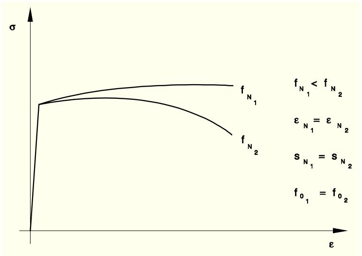
| ε | f_N1 | f_N2 | |-------|-------|-------| | 0 | 0 | 0 | | >0 | >0 | >0 |

# Integration of the elastoplastic equations The integration of the elastoplastic equations for the porous plasticity model is carried out using the backward Euler scheme proposed by Aravas (1987). This method is briefly discussed in the following paragraphs; the user can refer to the paper for further details. During the constitutive calculations in an increment, the stress and state variables are known at time t (beginning of the increment). Given a total incremental strain $\Delta \varepsilon ,$ , the stress and state variables need to be updated at $t + \Delta t$ (end of the increment) so that they satisfy the yield condition, flow rules, and evolution equation of the state variables. To do this, consider the elasticity equations Equation 4.3.6-1 $$ \pmb {\sigma} = \mathbf {D} ^ {e l}: \pmb {\varepsilon} ^ {e l} = \mathbf {D} ^ {e l}: (\pmb {\varepsilon} ^ {e l} | _ {t} + \Delta \pmb {\varepsilon} ^ {e l}) = \pmb {\sigma} ^ {e l} - \mathbf {D} ^ {e l}: \Delta \pmb {\varepsilon} ^ {p l}, $$ where $$ \pmb {\sigma} ^ {e l} = \mathbf {D} ^ {e l}: (\pmb {\varepsilon} ^ {e l} | _ {t} + \Delta \pmb {\varepsilon}) $$ is the elastic predictor and $$ \mathbf {D} ^ {e l} = 2 G \mathfrak {I} + \left(K - \frac {2}{3} G\right) \mathbf {I I} $$ is the linear isotropic elasticity tensor with G and K being the shear and bulk modulus, respectively, and = and I being the fourth- and second-order identity tensors, respectively. Also, in the above, the additive decomposition of strain is used to write the total incremental strain as the sum of the elastic and plastic parts. All of the stress and state variables are evaluated at $t + \Delta t$ unless indicated otherwise. The yield condition, the flow rule, and the evolution of the state variables are rewritten as $$ \phi (\pmb {\sigma}, H ^ {\alpha}) = 0, $$ $$ \Delta \pmb {\varepsilon} ^ {p l} = \frac {1}{3} \Delta \varepsilon_ {p} \mathbf {I} + \Delta \varepsilon_ {q} \mathbf {n}, $$ Equation 4.3.6-2 and $$ \Delta H ^ {\alpha} = \bar {H} ^ {\alpha} (\Delta \pmb {\varepsilon} ^ {p l}, \pmb {\sigma}, H ^ {\beta}), $$ Equation 4.3.6-3 where $$ \mathbf {n} = \frac {3}{2 q} \mathbf {S}, $$ $$ \Delta \varepsilon_ {p} = - \Delta \lambda \frac {\partial \phi}{\partial p}, $$ $$ \Delta \varepsilon_ {q} = \Delta \lambda \frac {\partial \phi}{\partial q}. $$ In the above $H ^ { \alpha } , \alpha = 1 , 2$ are the state variables $\bar { \varepsilon } _ { m } ^ { p l }$ and $f ,$ respectively. The plastic multiplier $\Delta \lambda$ is eliminated from the last two equations to give $$ \Delta \varepsilon_ {p} \frac {\partial \phi}{\partial q} + \Delta \varepsilon_ {q} \frac {\partial \phi}{\partial p} = 0. $$ Equation 4.3.6-2 is used in the elasticity Equation 4.3.6-1 to yield Equation 4.3.6-4 $$ \pmb {\sigma} = \pmb {\sigma} ^ {e l} - K \Delta \varepsilon_ {p} \mathbf {I} - 2 G \Delta \varepsilon_ {q} \mathbf {n}. $$ ${ \bf S } ^ { e l }$ and n are coaxial; therefore, n is determined as Equation 4.3.6-5 $$ \mathbf {n} = \frac {3}{2 q ^ {e l}} \mathbf {S} ^ {e l}. $$ Once n is known, it is easily seen that consistent determination of the scalars $\Delta \varepsilon _ { p }$ and $\Delta \varepsilon _ { q }$ completes the solution. Therefore, the problem of integrating the pressure-dependent elastoplastic constitutive equations is reduced to solving the following two nonlinear equations for the scalars $\Delta \varepsilon _ { p }$ and $\Delta \varepsilon _ { q }$ : Equation 4.3.6-6 $$ \phi (p, q, H ^ {\alpha}) = 0, $$ Equation 4.3.6-7 $$ \Delta \varepsilon_ {p} \frac {\partial \phi}{\partial q} + \Delta \varepsilon_ {q} \frac {\partial \phi}{\partial p} = 0. $$ In the above equations $p , q ,$ , and $H ^ { \alpha }$ are defined by Equation 4.3.6-8 $$ p = p ^ {e l} + K \Delta \varepsilon_ {p}, $$ Equation 4.3.6-9 $$ q = q ^ {e l} - 3 G \Delta \varepsilon_ {q}, $$ Equation 4.3.6-10 $$ \Delta H ^ {\alpha} = h ^ {\alpha} (\Delta \varepsilon_ {p}, \Delta \varepsilon_ {q}, p, q, H ^ {\beta}), $$ where Equation 4.3.6-8 and Equation 4.3.6-9 are obtained by projecting Equation 4.3.6-4 onto I and n, respectively, and Equation 4.3.6-10 is an alternate form of Equation 4.3.6-3. Solving the above system of equations for the unknowns $p , q , \Delta \varepsilon _ { p } , \Delta \varepsilon _ { q }$ ; and $H ^ { \alpha }$ completes the integration algorithm for the porous plasticity model. Equation 4.3.6-6 and Equation 4.3.6-7 are solved for $\Delta \varepsilon _ { p }$ and $\Delta \varepsilon _ { q }$ using Newton's method; p and q are updated using Equation 4.3.6-8 and Equation 4.3.6-9; the state variables are updated using Equation 4.3.6-10. # Computing the linearization moduli In the implicit finite element method of solving large-deformation problems, the discretized equilibrium equations result in a set of nonlinear equations for the nodal unknowns at the end of the increment. ABAQUS/Standard uses Newton's method to solve these equations, which requires the computation of linearization moduli $$ \mathcal {J} = \frac {\partial \Delta \pmb {\sigma}}{\partial \Delta \pmb {\varepsilon}} = \left(\frac {\partial \pmb {\sigma}}{\partial \pmb {\varepsilon}}\right) _ {t + \Delta t}. $$ To compute $\mathcal { I }$ (also known as the Jacobian), we start with the elasticity equations ( Equation 4.3.6-4), which can be rewritten as $$ \pmb {\sigma} = 2 G (\mathbf {e} ^ {e l} | _ {t} + \Delta \mathbf {e} - \Delta \varepsilon_ {q} \mathbf {n}) + K (\varepsilon_ {k k} ^ {e l} | _ {t} + \Delta \varepsilon_ {k k} - \Delta \varepsilon_ {p}) \mathbf {I}, $$ where $\mathbf { e } = \pmb { \varepsilon } - ( 1 / 3 ) \varepsilon _ { k k } \mathbf { I }$ is the deviatoric part of ". From the above equation you find that Equation 4.3.6-11 $$ \partial \pmb {\sigma} = 2 G (\partial \mathbf {e} - \partial \Delta \varepsilon_ {q} \mathbf {n} - \Delta \varepsilon_ {q} \partial \mathbf {n}) + K (\partial \varepsilon_ {k k} - \partial \Delta \varepsilon_ {p}) \mathbf {I}. $$ Once again Equation 4.3.6-6 and Equation 4.3.6-7 are used in computing the variations $\partial \Delta \varepsilon _ { p }$ and $\partial \Delta \varepsilon _ { q }$ . After some lengthy algebraic calculations, a set of linear equations is obtained that can be solved for $\partial \Delta \varepsilon _ { p }$ and $\partial \Delta \varepsilon _ { q }$ . These derivatives are substituted into Equation 4.3.6-11 to obtain the linearization moduli. In general this linearization moduli is not symmetric. Further details of the derivation of the Jacobian can be found in Aravas (1987). # 4.3.7 Cast iron plasticity The cast iron plasticity constitutive model is intended for modeling the elastoplastic behavior of gray cast iron. In tension gray cast iron is more brittle than most metals. This brittleness is attributed to the microstructure of the material, which consists of a distribution of graphite flakes in a steel matrix. In tension the graphite flakes act as stress concentrators, leading to an overall decrease in mechanical properties (such as yield strength). In compression, on the other hand, the graphite flakes serve to transmit stresses, and the overall response is governed by the response of the steel matrix alone. The above differences manifest themselves in the following macroscopic properties: (i) different yield strengths in tension and compression, with the yield stress in compression being a factor of three or more higher than the yield stress in tension; (ii) inelastic volume change in tension, but little or no inelastic volume change in compression; and (iii) different hardening behavior in tension and compression. It is commonly accepted (Hjelm, 1992, 1994) that a Mises-type yield condition along with an associated flow rule models the material response sufficiently accurately under compressive loading conditions. This assumption is not true for tensile loading conditions: a pressure-dependent yield surface with nonassociated flow is required to model the brittle behavior in tension. The model is described in detail in the remainder of this section. # Strain rate decomposition An additive strain rate decomposition is assumed: $$ \dot {\varepsilon} = \dot {\varepsilon} ^ {e l} + \dot {\varepsilon} ^ {p l}, $$ where "\_ is the total strain rate, $\dot { \pmb { \varepsilon } } ^ { e l }$ is the elastic part of the strain rate, and $\dot { \varepsilon } ^ { p l }$ is the inelastic (plastic) part of the strain rate. # Elastic behavior In compression the elastic behavior of gray cast iron is similar to that of many steels. It shows a well-defined elastic stiffness. In uniaxial tension the slope of the stress/strain curve decreases continuously, and it is difficult to estimate the elastic modulus from experimental results. The model in ABAQUS assumes that the elastic behavior of gray cast iron can be represented by linear isotropic elasticity, with the same stiffness in tension and compression. # Yield condition The model makes use of a composite yield surface to describe the different behavior in tension and compression. In tension yielding is assumed to be governed by the maximum principal stress, while in compression yielding is assumed to be pressure-independent and governed by the deviatoric stresses alone. In principal stress space the composite yield surface consists of the Rankine cube in tension and the Mises cylinder in compression. The material is assumed to be isotropic; hence, the yield surface can be expressed as a function of three invariant measures of the stress tensor: the equivalent pressure stress, $$ p = - \frac {1}{3} \pmb {\sigma}: \mathbf {I}; $$ the Mises equivalent stress, $$ q = \sqrt {\frac {3}{2} \mathbf {S} : \mathbf {S}}; $$ and the third invariant of the deviatoric stress, $$ r = (\frac {9}{2} \mathbf {S} \cdot \mathbf {S}: \mathbf {S}) ^ {\frac {1}{3}}, $$ where S is the stress deviator, defined as $$ \mathbf {S} = p \mathbf {I} + \pmb {\sigma}, $$ $\pmb { \sigma }$ is the Cauchy stress tensor, and I is the second-order identity tensor. It is convenient to combine the invariants q and r to define a nondimensional quantity, £, where $$ \cos (3 \Theta) = (\frac {r}{q}) ^ {3}. $$ In principal stress space the variable £ identifies the meridional plane for a given stress state. On any given meridional plane the yield surface consists of two distinct line segments given by $$ F _ {t} = R _ {R} (\Theta) q - p - \sigma_ {t} = 0 $$ and $$ F _ {c} = q - \sigma_ {c} = 0. 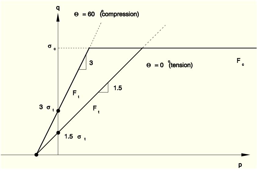$$ In the expressions above $R _ { R } ( \Theta ) = ( 2 / 3 )$ cos $\Theta ; \sigma _ { t } ( \bar { \varepsilon } _ { t } ^ { p l } , \theta , f ^ { \alpha } )$ is the yield stress in uniaxial tension, which may depend on the equivalent plastic strain in uniaxial tension $\bar { \varepsilon } _ { t } ^ { p l }$ , temperature $\theta ,$ and field variables $f ^ { \alpha } \left( \alpha = 1 , 2 , . . \right) ;$ and $\sigma _ { c } ( \bar { \varepsilon } _ { c } ^ { p l } , \theta , f ^ { \alpha } )$ is the yield stress in uniaxial compression, which may depend on the equivalent plastic strain in uniaxial compression $\bar { \varepsilon } _ { c } ^ { p l }$ , temperature $\theta ,$ and field variables $f ^ { \alpha } \left( \alpha = 1 , 2 , . . \right)$ . The composite yield surface is illustrated in the meridional plane in Figure 4.3.7-1, in the deviatoric plane in Figure 4.3.7-2, and in the principal stress space in Figure 4.3.7-3. Figure 4.3.7-1 Schematic of the yield surface in the meridional plane. 

line

| p | q (θ = 60°, compression) | q (θ = 0°, tension) | |------|---------------------------|----------------------| | 0 | 0 | 0 | | 3 | 3 | 1.5 | | 0 | 0 | 1.5 |

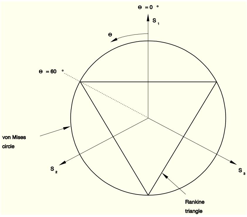
Figure 4.3.7-2 Schematic of the yield surface in the deviatoric plane. 

text_image

Θ = 0 ° S₁ Θ Θ = 60 ° von Mises circle S₂ S₃ Rankine triangle

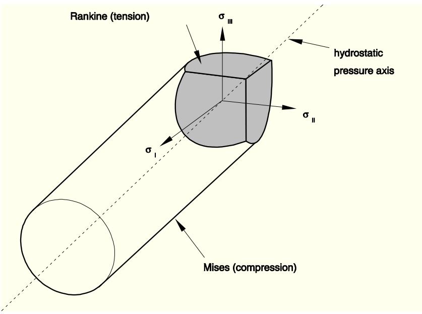
Figure 4.3.7-3 Schematic of the yield surface in the principal stress space. 

text_image

Rankine (tension) σⅢ hydrostatic pressure axis σⅡ σⅠ Mises (compression)

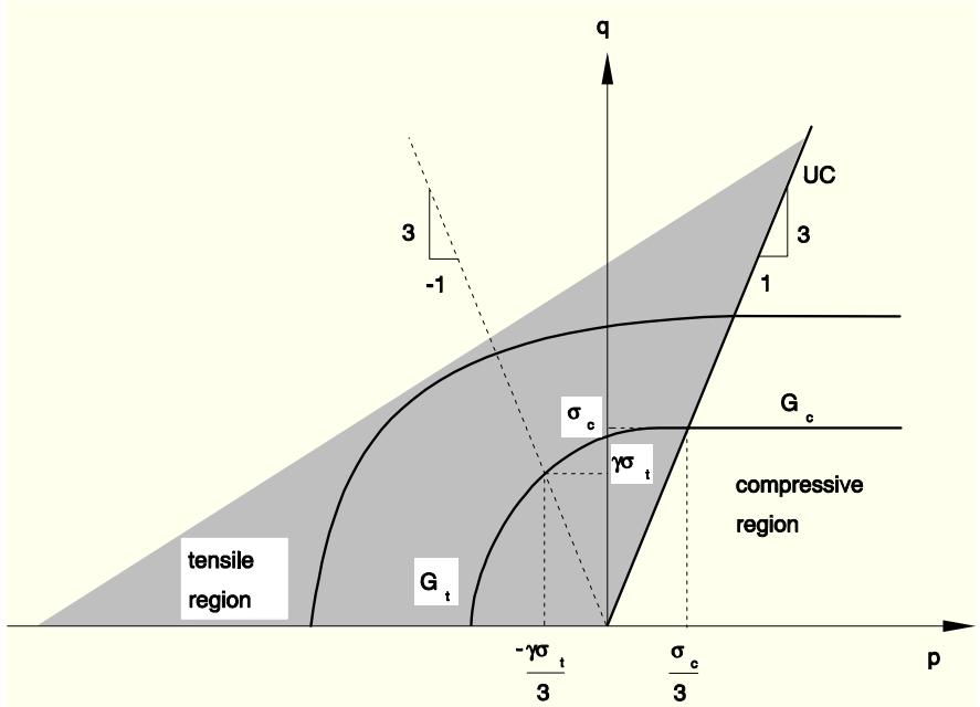
# Flow rule For the purposes of discussing the flow and hardening behavior, it is useful to divide a meridional plane into two regions as shown in Figure 4.3.7-4. Figure 4.3.7-4 Schematic of the flow potentials in the meridional plane. 

text_image

q UC 3 -1 1 G_c σ_c γσ_t compressive region tensile region G_t -γσ_t/3 σ_c/3 p

The region to the left of the uniaxial compression line (labeled UC) is referred to as the "tensile region," and the region to the right of the uniaxial compression line is referred to as the "compressive region." The plastic strains are defined to be normal to a family of self-similar flow potentials parametrized by the value of the potential G: $$ \dot {\pmb {\varepsilon}} ^ {p l} = \dot {\lambda} \frac {\partial G}{\partial \pmb {\sigma}}, $$ where $\dot { \lambda }$ is the nonnegative plastic multiplier. The flow potential, $G ( p , q , \theta , f ^ { \alpha } )$ , is assumed to be independent of the third stress invariant (independent of £). It consists of the Mises cylinder in compression with an ellipsoidal "cap" in tension. The transition between the two surfaces is smooth. The projection of the flow potential onto the deviatoric plane is a circle. On the meridional plane the potential G can take one of two values, $G _ { t }$ and $G _ { c }$ , defined by the relations $$ \frac {(p - G _ {t}) ^ {2}}{a ^ {2}} + q ^ {2} = 9 G _ {t} ^ {2} \quad \mathrm{when} \quad p < \frac {\sigma_ {c}}{3}, $$ $$ q = 3 G _ {c} \quad \text {when} \quad p \geq \frac {\sigma_ {c}}{3}. $$ $G _ { t }$ is the value of the potential in the tensile region, and $G _ { c }$ is the value of the potential in the compressive region. The potential in the tensile region is of the form of an ellipse, where a is the ratio of the horizontal (p) to the vertical (q) axis of the ellipse. The shape of the ellipse is controlled by $^ { a , }$ which is chosen such that it passes through the two points $\smash { \big ( - \gamma \sigma _ { t } / 3 , \gamma \sigma _ { t } \big ) }$ and $( \sigma _ { c } / 3 , \sigma _ { c } )$ , where $\gamma$ is a material parameter that controls plastic dilatation. The above requirement determines $a ^ { 2 }$ to be equal to $( \sigma _ { c } + \gamma \sigma _ { t } ) / 9 ( \sigma _ { c } - \gamma \sigma _ { t } )$ . The value of the potential, G, depends on the current stress point $( p , q )$ . In the compressive region the flow potential consists of the Mises straight line. A consequence of the above choice of the flow potential is that plastic flow results in inelastic volume change in the tensile region and no inelastic volume change in the compressive region. Figure 4.3.7-4 illustrates two potentials in the $p – q$ plane. It can be shown that for uniaxial tension, $\gamma = 2 r _ { c t } ( 1 + \nu _ { p l } ) / 3$ , where $r _ { c t } = \sigma _ { c } / \sigma _ { t }$ and $\nu _ { p l }$ (referred to as the "plastic Poisson's ratio") is equal to the absolute value of the ratio of the transverse to the longitudinal plastic strain under uniaxial tension. The quantities $\sigma _ { c } , \sigma _ { t }$ , and $\nu _ { p l }$ are material properties that must be provided by the user. The plastic Poisson's ratio, $\nu _ { p l }$ , is expected to be less than 0:5 since experiments suggest that there is a permanent increase in the volume of gray cast iron when it is loaded in uniaxial tension beyond yield. In addition, $\nu _ { p l }$ must be greater than ¡1 for the potential to be well-defined. For the gray cast iron described in the work of Coffin (1950), the value of $\nu _ { p l }$ is approximately 0:04. This estimate is based on the reported value of the permanent volume change close to the ultimate tensile stress. The value of $\nu _ { p l }$ may change with plastic deformation. However, the model in ABAQUS assumes that it is constant with respect to plastic deformation. It can depend on temperature and field variables. Since the flow potential is different from the yield surface (nonassociated flow), the material Jacobian matrix is unsymmetric. # Hardening ABAQUS assumes that the graphite flakes do not influence the hardening behavior in the compressive region, where the matrix behavior (Mises plasticity) characterizes the overall response. In the tensile region the plastic strain consists of both a volumetric part (corresponding to opening up of the graphite flakes) and a deviatoric part (corresponding to inelastic shearing of the matrix). In the limiting case of pure hydrostatic tension it can be expected that the matrix material does not respond plastically; therefore, the entire plastic strain is volumetric, corresponding to the opening up of the graphite flakes. Thus, in the tensile region, we expect that the deviatoric part of the plastic strain decreases as the loading path approaches hydrostatic tension, eventually becoming zero at hydrostatic tension, while the volumetric part of the plastic strain decreases as the loading path approaches uniaxial compression and is zero for uniaxial compression and confining pressures higher than $\sigma _ { c } / 3$ . The hardening of the model is controlled by the evolution of $\sigma _ { t } = \sigma _ { t } ( \bar { \varepsilon } _ { t } ^ { p l } , \theta , f ^ { \alpha } )$ and $\sigma _ { c } = \sigma _ { c } ( \bar { \varepsilon } _ { c } ^ { p l } , \theta , f ^ { \alpha } )$ . To develop the hardening model, we need to find expressions for the equivalent plastic strains, $\bar { \varepsilon } _ { t } ^ { p l }$ and $\bar { \varepsilon } _ { c } ^ { p l }$ , as functions of the plastic strain tensor $\varepsilon ^ { p l }$ . To simplify the discussion, we assume that the temperature µ and the field variables $f ^ { \alpha } \left( \alpha = 1 , 2 , . . \right)$ are constants, so that the yield stresses are taken to be functions of the corresponding equivalent strains only. Furthermore, it is convenient to decompose the plastic strain rate into volumetric and deviatoric components: $$ \dot {\varepsilon} _ {v o l} ^ {p l} = \dot {\pmb {\varepsilon}} ^ {p l}: \mathbf {I}, $$ $$ \dot {e} ^ {p l} = \frac {2}{3} \dot {\varepsilon} ^ {p l}: \mathbf {n}, $$ where $\mathbf { n } = ( 3 / 2 q ) \mathbf { S }$ is the flow direction in the deviatoric plane. To find an expression relating $\bar { \varepsilon } _ { c } ^ { p l }$ to $\varepsilon ^ { p l }$ , we use the equivalent plastic work expression $$ \sigma_ {c} \dot {\bar {\varepsilon}} _ {c} ^ {p l} = \pmb {\sigma}: \dot {\pmb {\varepsilon}} ^ {p l}. $$ Using the definition of the flow potential, it then follows (given that $\dot { \varepsilon } _ { v o l } ^ { p l } = 0$ and $q = \sigma _ { c }$ in compression) that $$ \dot {\bar {\varepsilon}} _ {c} ^ {p l} = \dot {e} ^ {p l}. $$ This expression is used to update $\sigma _ { c } ( \bar { \varepsilon } _ { c } ^ { p l } )$ for all loading conditions, including tensile loading conditions. Next, we find an expression relating $\bar { \varepsilon } _ { t } ^ { p l }$ to $\varepsilon ^ { p l }$ . Using the equivalent plastic work expression $$ \sigma_ {t} \dot {\bar {\varepsilon}} _ {t} ^ {p l} = \pmb {\sigma}: \dot {\pmb {\varepsilon}} ^ {p l} $$ and the definition of the flow potential, it follows that $$ \dot {\bar {\varepsilon}} _ {t} ^ {p l} = \frac {1}{\sigma_ {t}} (- p \dot {\varepsilon} _ {v o l} ^ {p l} + q \dot {e} ^ {p l}). $$ This expression is used to update the yield stress $\sigma _ { t } ( \bar { \varepsilon } _ { t } ^ { p l } )$ for all loading conditions, including compressive loading conditions. 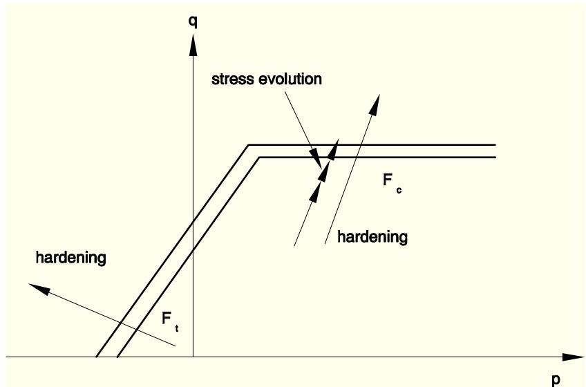Under predominantly compressive loading conditions, $\dot { \varepsilon } _ { v o l } ^ { p l } = 0 , \dot { \bar { \varepsilon } } _ { c } ^ { p l } = \dot { e } ^ { p l }$ , and $\dot { \bar { \varepsilon } } _ { t } ^ { p l } = ( \sigma _ { c } / \sigma _ { t } ) \dot { e } ^ { p l }$ . Thus, both $\sigma _ { c }$ and $\sigma _ { t }$ are updated based on the deviatoric plastic strain, $e ^ { p l }$ , alone. This behavior is depicted in Figure 4.3.7-5. Figure 4.3.7-5 Hardening during compression loading. 

text_image

q stress evolution F_c hardening hardening F_t p

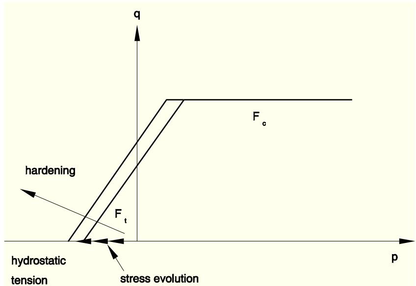
At the other extreme, under hydrostatic tension (see Figure 4.3.7-6) $\dot { e } ^ { p l } = 0$ . Figure 4.3.7-6 Hardening due to hydrostatic tension $( p < 0$ and $q = 0 )$ . 

text_image

q F_c hardening F_t hydrostatic tension stress evolution p

Hence, $\dot { \bar { \varepsilon } } _ { c } ^ { p l } = 0 ;$ , and $\dot { \bar { \varepsilon } } _ { t } ^ { p l } = \dot { \varepsilon } _ { v o l } ^ { p l }$ . Consequently, $\sigma _ { c }$ does not evolve, but $\sigma _ { t }$ evolves based on $\dot { \varepsilon } _ { v o l } ^ { p l }$ . For all other loading paths in the tensile region, both $\dot { \varepsilon } _ { v o l } ^ { p l }$ and $\dot { e } ^ { p l }$ are nonzero. In such cases $\sigma _ { c }$ is updated based on the deviatoric plastic strain, $e ^ { p l }$ , alone, while $\sigma _ { t }$ is updated based on both $\varepsilon _ { v o l } ^ { p l }$ and $e ^ { p l }$ (see Figure 4.3.7-5). Given the micromechanics of deformation of gray cast iron, the behavior seems