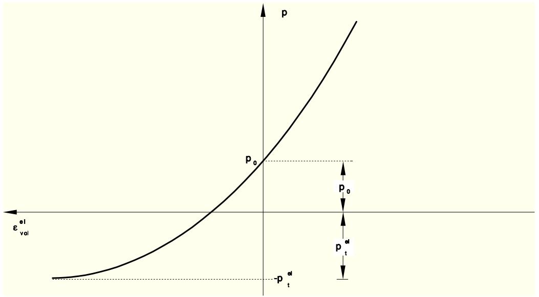
Figure 4.4.1-1 Porous elastic volumetric behavior. 

line

| ε_vol^el | p | | -------- | ------- | | - | - | | 0 | p₀ | | ε_vol^el | -p_t^el |

The deviatoric elastic behavior is defined either by choosing a constant shear modulus, $G ,$ so that the deviatoric elastic stiffness is independent of the equivalent pressure stress or choosing a constant Poisson's ratio, $\nu ,$ so that the deviatoric elastic stiffness increases as the equivalent pressure stress increases. If a constant shear modulus is given, the deviatoric relationship is $$ \mathbf {S} = 2 G \mathbf {e} ^ {e l}, $$ whereas when Poisson's ratio is given, the relationship has the rate form $$ d \mathbf {S} = 2 \hat {G} d \mathbf {e} ^ {e l}, $$ where Equation 4.4.1-6 $$ \hat {G} = \frac {3 (1 - 2 \nu) (1 + e _ {0})}{2 (1 + \nu) \kappa} (p + p _ {t} ^ {e l}) \exp (\varepsilon_ {v o l} ^ {e l}) $$ for a material with nonzero tensile strength. In these equations S is the deviatoric stress: $$ \mathbf {S} = \boldsymbol {\sigma} + p \mathbf {I}, $$ and ${ \pmb { \mathrm { e } } } ^ { e l }$ is the deviatoric part of the elastic strain: $$ \mathbf {e} ^ {e l} = \pmb {\varepsilon} ^ {e l} - \frac {1}{3} \varepsilon_ {v o l} ^ {e l} \mathbf {I}, $$ $\varepsilon _ { v o l } ^ { e l }$ is the volumetric part of the elastic strain. # 4.4.2 Models for granular or polymer behavior The behavior of granular and polymeric materials is complex. However, under essentially monotonic loading conditions rather simple constitutive models provide useful design information. These constitutive models are essentially pressure-dependent plasticity models that have historically been popular in the geotechnical engineering field. However, more recently they have also been found to be useful for the modeling of some polymeric and composite materials that exhibit significantly different yield behavior in tension and compression. The models described here are extensions of the original Drucker-Prager model ( Drucker and Prager, 1952). In the context of geotechnical materials the extensions of interest include the use of curved yield surfaces in the meridional plane, the use of noncircular yield surfaces in the deviatoric stress plane, and the use of nonassociated flow laws. In the context of polymeric and composite materials, the extensions of interest are mainly the use of nonassociated flow laws and the inclusion of rate-dependent effects. In both contexts the models have been extended to include creep. # Available yield criteria Three yield criteria are provided in this set of models. They offer differently shaped yield surfaces in the meridional plane (p-q plane): a linear form, a hyperbolic form, and a general exponent form (see Figure 4.4.2-1). Figure 4.4.2-1 Yield criteria in the meridional plane.  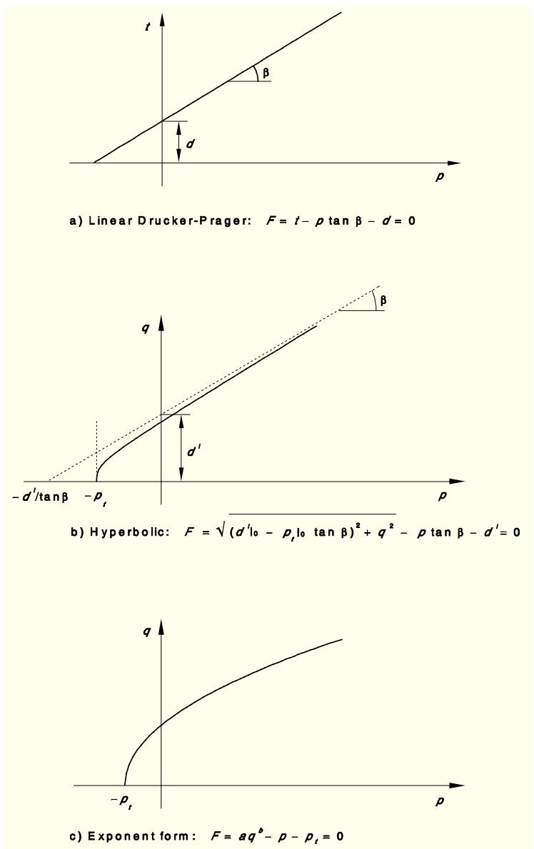The stress invariants used in the formulation are defined in \`\`Stress invariants,'' Section 1.5.3. The choice of model depends largely on the material, the experimental data available for calibration of the model parameters, and on the range of pressure stress values likely to be encountered. This choice is discussed in detail in \`\`Extended Drucker-Prager models,'' Section 11.3.1 of the ABAQUS/Standard User's Manual and \`\`Extended Drucker-Prager model,'' Section 10.3.1 of the ABAQUS/Explicit User's Manual. The linear model (available in ABAQUS/Standard and ABAQUS/Explicit) provides a noncircular section in the deviatoric (¦) plane, associated inelastic flow in the deviatoric plane, and separate dilation and friction angles. The smoothed surface used in the deviatoric plane differs from a true Mohr-Coulomb surface that exhibits vertices. This has restrictive implications, especially with respect to flow localization studies for granular materials, but this may not be of major significance in many routine design applications. Input data parameters define the shape of the yield and flow surfaces in the deviatoric plane as well as the friction and dilation angles, so that a range of simple theories is provided; for example, the original Drucker-Prager model (Drucker and Prager, 1952) is available within this model. The hyperbolic and general exponent models (available in ABAQUS/Standard only) use a von Mises (circular) section in the deviatoric stress plane with associated plastic flow. A hyperbolic flow potential is used in the meridional plane, which--in general--means nonassociated flow. # Hardening, rate dependence, and creep Perfect plasticity as well as isotropic hardening are offered with these models. Isotropic hardening is generally considered to be a suitable model for problems in which the plastic straining goes well beyond the incipient yield state where the Bauschinger effect is noticeable ( Rice, 1975). This hardening theory is, therefore, used for processes involving large plastic strain and in which the plastic strain rate does not continuously reverse direction sharply; that is, the models are intended for problems involving essentially monotonic loading, as distinct from cyclic loading. The isotropic hardening models can be used for rate-dependent as well as rate-independent behavior. The rate-dependent version is intended for relatively high strain rate applications. Isotropic hardening means that the yield function is written as $$ f (\pmb {\sigma}) = \bar {\sigma} (\bar {\varepsilon} ^ {p l}, \dot {\bar {\varepsilon}} ^ {p l}, \theta , f ^ {\alpha}), $$ where $f$ is an isotropic function of a symmetric second-order tensor and $\bar { \sigma }$ is the equivalent yield stress given by $$ \begin{array}{l} \bar {\sigma} = \sigma_ {c} (\bar {\varepsilon} ^ {p l}, \dot {\bar {\varepsilon}} ^ {p l}, \theta , f ^ {\alpha}) \quad \mathrm{ifhardeningisdefinedbytheuniaxialcompressionyieldstress}, \sigma_ {c}, \\ = \sigma_ {t} (\bar {\varepsilon} ^ {p l}, \dot {\bar {\varepsilon}} ^ {p l}, \theta , f ^ {\alpha}) \quad \mathrm{ifhardeningisdefinedbytheuniaxialtensionyieldstress}, \sigma_ {t}, \\ = d (\bar {\varepsilon} ^ {p l}, \dot {\bar {\varepsilon}} ^ {p l}, \theta , f ^ {\alpha}) \quad \text {if hardening is defined by the pure shear (cohesion) yield stress}, \\ \end{array} $$ where $\tau$ is the shear stress; $K$ is a material parameter; $\bar { \varepsilon } ^ { p l }$ is the equivalent plastic strain; $\dot { \bar { \varepsilon } } ^ { p l }$ is the equivalent plastic strain rate; $\theta$ is temperature; and $f ^ { \alpha } , \alpha = 1 , 2 .$ :: are other predefined field variables. The equivalent plastic strain rate, $\dot { \bar { \varepsilon } } ^ { p l }$ , is defined for the linear Drucker-Prager model as $$ \begin{array}{l} \dot {\varepsilon} ^ {p l} = \left| \dot {\epsilon} _ {1 1} ^ {p l} \right| \quad \text { if hardening is defined in uniaxial compression }, \\ = \dot {\epsilon} _ {1 1} ^ {p l} \quad \text { if hardening is defined in uniaxial tension }, \\ = \frac {\dot {\gamma} ^ {p l}}{\sqrt {3}} \quad \text { if hardening is defined in pure shear }, \\ \end{array} $$ where $\dot { \gamma } ^ { p l }$ is the engineering shear plastic strain rate and is defined for the hyperbolic and exponential Drucker-Prager models by the plastic work expression Equation 4.4.2-1 $$ \bar {\sigma} \dot {\bar {\varepsilon}} ^ {p l} = \pmb {\sigma}: \dot {\pmb {\varepsilon}} ^ {p l}. $$ The functional dependence $\bar { \sigma } ( \bar { \varepsilon } ^ { p l } , \dot { \bar { \varepsilon } } ^ { p l } , \theta , f ^ { \alpha } )$ includes hardening as well as rate-dependent effects and can be specified directly on the \*DRUCKER PRAGER HARDENING, RATE= option. The test data are entered as tables of yield stress values versus equivalent plastic strain at different equivalent plastic strain rates: one table per strain rate. The yield stress at a given strain and strain rate is interpolated directly from these tables. This option is useful when the shapes of the stress-strain curves are different at different strain rates. Alternatively, when it can be assumed that the shapes of the hardening curves at different strain rates are similar, the hardening dependence alone is specified on the \*DRUCKER PRAGER HARDENING option while the rate dependence is specified on the \*RATE DEPENDENT option. In this case we assume that the rate dependence can be written in a separable form: $$ \bar {\sigma} = R \sigma^ {0}, $$ where $\sigma ^ { 0 } ( \bar { \varepsilon } ^ { p l } , \theta , f ^ { \alpha } )$ is the static yield stress defined on the \*DRUCKER PRAGER HARDENING option and $R ( \dot { \bar { \varepsilon } } ^ { p l } , \theta , f ^ { \alpha } )$ scales this value at nonzero strain rate $( R = 1 . 0 \mathrm { a t } \dot { \bar { \varepsilon } } ^ { p l } = 0 . 0 )$ . The yield ratio R is defined on the \*RATE DEPENDENT option either in a tabular form or using the standard power law form $$ R = 1 + \left(\frac {\dot {\bar {\varepsilon}} ^ {p l}}{D}\right) ^ {\frac {1}{n}}, $$ where $D ( \theta , f ^ { \alpha } )$ and $n ( \theta , f ^ { \alpha } )$ are material parameters. Creep models are most suitable for applications that exhibit time-dependent inelastic deformation at low deformation rates. Such inelastic deformation, which can coexist with rate-independent plastic deformation, is described later in this section. However, the existence of creep in an ABAQUS material definition precludes the use of rate dependence as described above. # Strain rate decomposition An additive strain rate decomposition is assumed: Equation 4.4.2-2 $$ d \pmb {\varepsilon} = d \pmb {\varepsilon} ^ {e l} + d \pmb {\varepsilon} ^ {p l} + d \pmb {\varepsilon} ^ {c r}, $$ where d" is the total strain rate, $d \pmb { \varepsilon } ^ { e l }$ is the elastic strain rate, $d \pmb { \varepsilon } ^ { p l }$ is the inelastic (plastic) strain rate, and $d \varepsilon ^ { c r }$ is the inelastic creep strain rate. The term $d \varepsilon ^ { p l }$ is omitted if the stress point is inside the yield surface, and the term $d \pmb { \varepsilon } ^ { c r }$ is omitted if creep has not been defined or is not active. # Elastic behavior The elastic behavior can be modeled as linear or with the porous elasticity model including tensile strength described in \`\`Porous elasticity,'' Section 4.4.1. If creep has been defined, the elastic behavior must be modeled as linear. 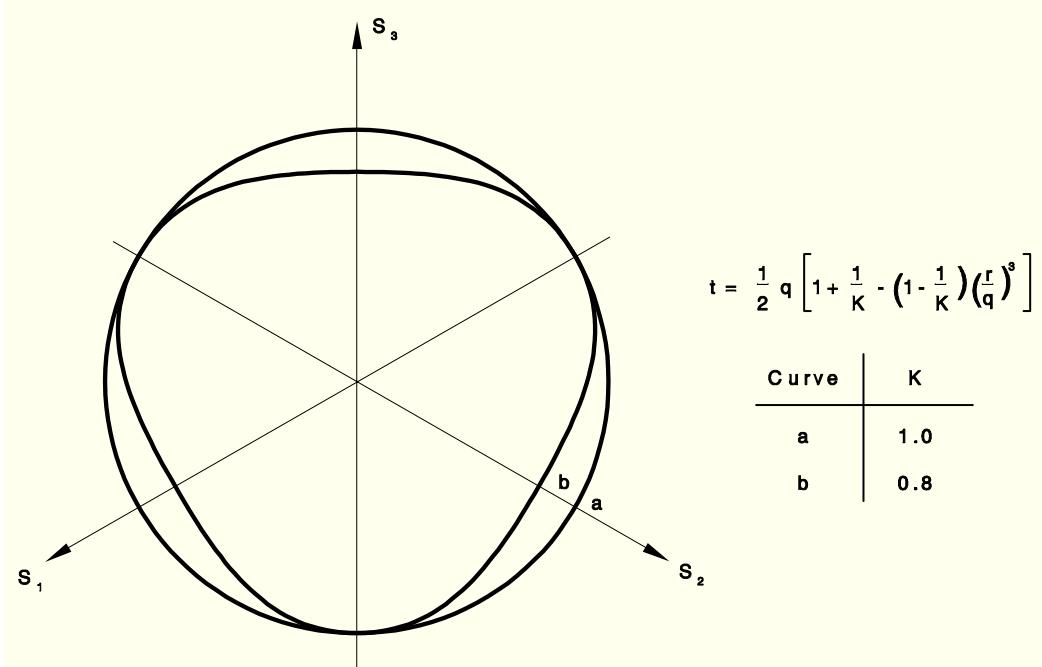# Linear Drucker-Prager model In this model we define a deviatoric stress measure $$ t = \frac {q}{2} \left[ 1 + \frac {1}{K} - \left(1 - \frac {1}{K}\right) \left(\frac {r}{q}\right) ^ {3} \right], $$ where $K ( \theta , f _ { \alpha } )$ is a material parameter. To ensure convexity of the yield surface, $0 . 7 7 8 \leq K \leq 1 . 0$ . This measure of deviatoric stress is used because it allows the matching of different stress values in tension and compression in the deviatoric plane, thereby providing flexibility in fitting experimental results when the material exhibits different yield values in triaxial tension and compression tests. This function is sketched in Figure 4.4.2-2. Figure 4.4.2-2 Typical yield surfaces for the linear model in the deviatoric plane. 

radar

| Curve | K | |-------|-----| | a | 1.0 | | b | 0.8 |

It only provides a coarse match to Mohr-Coulomb behavior (where the yield is independent of the intermediate principal stress). Since $( r / q ) ^ { 3 } = 1$ in uniaxial tension, $t = q / K$ in this case; since $( r / q ) ^ { 3 } = - 1$ in uniaxial compression, $t = q$ in that case. When $K = 1$ , the dependence on the third deviatoric stress invariant is removed; the Mises circle is recovered in the deviatoric plane: $t = q$ . With this expression for the deviatoric stress measure, the yield surface is defined as Equation 4.4.2-3 $$ F = t - p \tan \beta - d = 0, $$ where # Mechanical Constitutive Theories $d = ( 1 - \frac { 1 } { 3 } \tan \beta ) \sigma _ { c }$ if hardening is de¯ned by the uniaxial compression yield stress ; $\sigma _ { c } ;$ $= ( \frac { 1 } { K } + \frac { 1 } { 3 } \tan \beta ) \sigma _ { t }$ if hardening is de¯ned by the uniaxial tension yield stress ; $\sigma _ { t } .$ ; $= d$ if hardening is de¯ned by the shear (cohesion) yield stress ; $d ;$ and $\beta ( \theta , f ^ { \alpha } )$ is the friction angle of the material in the meridional stress plane. In the case of hardening defined in uniaxial compression, the linear yield criterion precludes friction angles $\beta > 7 1 . 5 ^ { \circ }$ (tan $\beta > 3 )$ . This is not seen as a limitation since it is unlikely this will be the case for real materials. 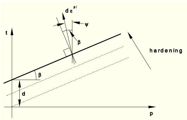The hardening parameter $d ( \bar { \sigma } )$ measures the cohesion of the material and represents isotropic hardening, as illustrated in Figure 4.4.2-3. Figure 4.4.2-3 Schematic of hardening and flow for the linear model in the $p { - } t$ plane. 

text_image

d ε^p1 ψ β β d hardening p t

The formulation treats $\beta$ as constant with respect to stress, although it is straightforward to extend the theory to provide for the functional dependence of $\beta$ on quantities such as $p .$ In \`\`Extended Drucker-Prager models,'' Section 11.3.1 of the ABAQUS/Standard User's Manual and \`\`Extended Drucker-Prager model,'' Section 10.3.1 of the ABAQUS/Explicit User's Manual, we describe a method for converting Mohr-Coulomb data $( \phi ,$ the angle of Coulomb friction, and $c ,$ the cohesion) to appropriate values of $\beta$ and $d .$ # Flow rule Potential flow in the linear model is assumed, so that Equation 4.4.2-4 $$ d \varepsilon^ {p l} = \frac {d \bar {\varepsilon} ^ {p l}}{c} \frac {\partial G}{\partial \pmb {\sigma}}, $$ where $c = ( 1 - \frac { 1 } { 3 } \tan \psi )$ if hardening is de¯ned in uniaxial compression ; = ( 1K + $= ( \frac { 1 } { K } + \frac { 1 } { 3 } \tan \psi )$ if hardening is de¯ned in uniaxial tension ; = 1 (1 + 1 $= \frac { 1 } { 2 } ( 1 + \frac { 1 } { K } )$ if hardening is de¯ned in pure shear (cohesion) ; and $$ \begin{array}{l} d \bar {\varepsilon} ^ {p l} = | d \epsilon_ {1 1} ^ {p l} | \quad \text { in the uniaxial compression case }, \\ = d \epsilon_ {1 1} ^ {p l} \quad \text { in the uniaxial tension case }, \\ = \frac {d \gamma^ {p l}}{\sqrt {3}} \quad \text { in the pure shear case, where } \gamma^ {p l} \text { is the engineering shear plastic strain. } \\ \end{array} $$ G is the flow potential, chosen in this model as Equation 4.4.2-5 $$ G = t - p \tan \psi , $$ where $\psi ( \theta , f ^ { \alpha } )$ is the dilation angle in the p-t plane. A geometrical interpretation of $\psi$ is shown in the t-p diagram of Figure 4.4.2-3. In the case of hardening defined in uniaxial compression, this flow rule definition precludes dilation angles $\psi > 7 1 . 5 ^ { \circ } ( \tan \psi > 3 )$ . This is not seen as a limitation since it is unlikely this will be the case for real materials. Comparison of Equation 4.4.2-3 and Equation 4.4.2-5 shows that the flow is associated in the deviatoric plane, because the yield surface and the flow potential both have the same functional dependence on t. However, the dilation angle, Ã, and the material friction angle, $\beta ,$ , may be different, so the model may not be associated in the $p { - } t$ plane. For $\psi = 0$ the material is nondilational; and if $\psi = \beta ;$ , the model is fully associated--the model is then of the type first introduced by Drucker and Prager (1952). For $\psi = \beta$ and $K = 1$ the original Drucker-Prager model is recovered. # Hyperbolic and general exponent models The hyperbolic and general exponent models, which are only available in ABAQUS/Standard, are written in terms of the first two stress invariants only. The hyperbolic yield criterion is a continuous combination of the maximum tensile stress condition of Rankine (tensile cut-off) and the linear Drucker-Prager condition at high confining stress. 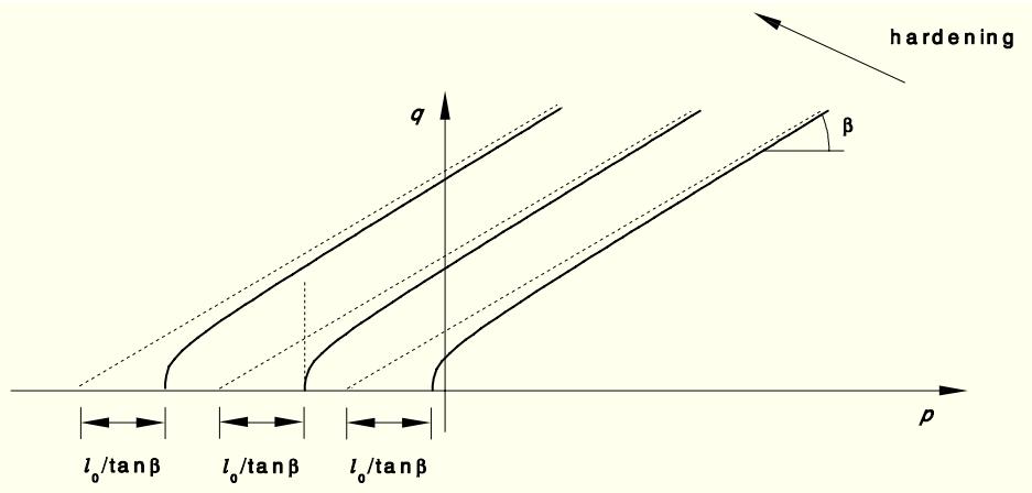It is written as Equation 4.4.2-6 $$ F = \sqrt {l _ {0} ^ {2} + q ^ {2}} - p \tan \beta - d ^ {\prime} = 0, $$ where $l _ { 0 } = ( d ^ { \prime } | _ { 0 } - p _ { t } | _ { 0 }$ tan $\beta ) , p _ { t } | _ { 0 }$ is the initial hydrostatic tension strength of the material, $d ^ { \prime } | _ { 0 }$ is the initial value of $d ^ { \prime }$ , and $\beta ( \theta , f ^ { \alpha } )$ is the friction angle measured at high confining pressure, as shown in Figure 4.4.2-1(b). $d ^ { \prime } ( \bar { \sigma } )$ is the hardening parameter, which is obtained from test data: # Mechanical Constitutive Theories $d ^ { \prime } = \sqrt { l _ { 0 } ^ { 2 } + \sigma _ { c } { } ^ { 2 } - \frac { v _ { c } } { 3 } }$ tan $\beta$ if hardening is de¯ned by the uniaxial compression yield stress ; $\sigma _ { c } ;$ $= \sqrt { l _ { 0 } ^ { 2 } + { \sigma _ { t } } ^ { 2 } } + \frac { \sigma _ { t } } { 3 } \tan \beta$ if hardening is de¯ned by the uniaxial tension yield stress ; ${ } _ { \cdot \sigma _ { t } ; }$ $= \sqrt { l _ { 0 } ^ { 2 } + d ^ { 2 } }$ if hardening is de¯ned by the shear (cohesion) yield stress ; $, d .$ The isotropic hardening assumed in this model treats $\beta$ as constant with respect to stress and is depicted in Figure 4.4.2-4. Calibration of this model is described in \`\`Extended Drucker-Prager models,'' Section 11.3.1 of the ABAQUS/Standard User's Manual. Figure 4.4.2-4 Schematic diagram of hardening for the hyperbolic model in the p-q plane. 

text_image

hardening β q p l₀/tanβ l₀/tanβ l₀/tanβ

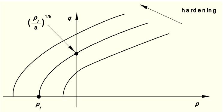
The general exponent form provides the most general yield criterion available in this class of models. The yield function is written as Equation 4.4.2-7 $$ F = a q ^ {b} - p - p _ {t} = 0, $$ where $a ( \theta , f ^ { \alpha } )$ and $b ( \theta , f ^ { \alpha } )$ are material parameters that are independent of plastic deformation and $p _ { t } ( \bar { \sigma } )$ is the hardening parameter that represents the hydrostatic tension strength of the material, as shown in Figure 4.4.2-1(c). $p _ { t } ( \bar { \sigma } )$ is related to test data as $p _ { t } = { a \sigma _ { c } } ^ { b } - \frac { \sigma _ { c } } { 3 }$ if hardening is de¯ned by the uniaxial compression yield stress ; $\sigma _ { c } ;$ = a¾t b + $= { a { \sigma _ { t } } ^ { b } } + { \frac { \sigma _ { t } } { 3 } }$ if hardening is de¯ned by the uniaxial tension yield stress ; $\sigma _ { t } \mathrm { : }$ ; $= a d ^ { b }$ if hardening is de¯ned by the shear (cohesion) yield stress ; $d .$ The isotropic hardening assumed in this model treats a and b as constant with respect to stress and is depicted in Figure 4.4.2-5. Figure 4.4.2-5 Schematic diagram of hardening for the general exponent model in the p-q plane. 

text_image

(p_t/a)^{1/b} q p_t hardening

The material parameters $a , b ,$ and $p _ { t }$ can be given directly; $\mathbf { o r } ,$ if triaxial test data at different levels of confining pressure are available, ABAQUS will determine the material parameters from the triaxial test data. A least squares fit, which minimizes the relative error in stress, is used to obtain the "best fit" values for $a , b ,$ and $p _ { t }$ . These and other calibration issues relating to this model are described in \`\`Extended Drucker-Prager models,'' Section 11.3.1 of the ABAQUS/Standard User's Manual. # Flow rule Potential flow in the hyperbolic and general exponent models is assumed, so that Equation 4.4.2-8 $$ d \varepsilon^ {p l} = \frac {d \bar {\varepsilon} ^ {p l}}{f} \frac {\partial G}{\partial \pmb {\sigma}}, $$ where f depends on how the hardening is defined (by uniaxial compression, uniaxial tension, or pure shear data) but can be written in general as $$ f = \frac {1}{\bar {\sigma}} \pmb {\sigma}: \frac {\partial G}{\partial \pmb {\sigma}}, $$ and $$ \begin{array}{l} d \bar {\varepsilon} ^ {p l} = | d \epsilon_ {1 1} ^ {p l} | \quad \text {in the uniaxial compression case}, \\ = d \epsilon_ {1 1} ^ {p l} \quad \mathrm{intheuniaialtensioncase}, \\ = \frac {d \gamma^ {p l}}{\sqrt {3}} \quad \mathrm{inthepureshearcase,where} \gamma^ {p l} \mathrm{istheengineeringshearplasticstrain.} \\ \end{array} $$ G is the flow potential, chosen in these models as a hyperbolic function: Equation 4.4.2-9 $$ G = \sqrt {(\epsilon \bar {\sigma} | _ {0} \tan \psi) ^ {2} + q ^ {2}} - p \tan \psi , $$ where $\psi ( \theta , f ^ { \alpha } )$ is the dilation angle measured in the $p – q$ plane at high confining pressure; $\bar { \sigma } | _ { 0 } = \bar { \sigma } | _ { \bar { \varepsilon } ^ { p l } = 0 , \dot { \bar { \varepsilon } } ^ { p l } = 0 }$ is the initial equivalent yield stress; and ² is a parameter, referred to as the eccentricity, that defines the rate at which the function approaches the asymptote (the flow potential tends to a straight line as the eccentricity tends to zero). This flow potential, which is continuous and