in turn for all components of $\overline{\mathbf{U}}$ . In the first application $\overline{\mathbf{U}} = \mathbf{e}_1$ , in the second application $\overline{\mathbf{U}} = \mathbf{e}_2$ , and so on, until in the $n$ th application $\overline{\mathbf{U}} = \mathbf{e}_n$ , so that the result is $$ \boxed {\mathbf {K U} = \mathbf {R}} \tag {4.17} $$ where we do not show the identity matrices $\mathbf{I}$ due to the virtual displacements on each side of the equation and $$ \boxed {\mathbf {R} = \mathbf {R} _ {B} + \mathbf {R} _ {S} - \mathbf {R} _ {I} + \mathbf {R} _ {C}} \tag {4.18} $$ and, as we shall do from now on, we denote the unknown nodal point displacements as $\mathbf{U}$ ; i.e., $\mathbf{U} \equiv \hat{\mathbf{U}}$ . The matrix K is the stiffness matrix of the element assemblage, $$ \boxed { \begin{array}{c} \mathbf {K} = \sum_ {m} \underbrace {\int_ {V ^ {(m)}} \mathbf {B} ^ {(m) T} \mathbf {C} ^ {(m)} \mathbf {B} ^ {(m)} d V ^ {(m)}} _ {= \mathbf {K} ^ {(m)}} \end{array} } \tag {4.19} $$ The load vector R includes the effect of the element body forces, $$ \boxed { \begin{array}{l} \mathbf {R} _ {B} = \sum_ {m} \underbrace {\int_ {V ^ {(m)}} \mathbf {H} ^ {(m) T} \mathbf {f} ^ {B (m)} d V ^ {(m)}} _ {= \mathbf {R} _ {B} ^ {(m)}} \end{array} } \tag {4.20} $$ the effect of the element surface forces, $$ \boxed { \begin{array}{l} \mathbf {R} _ {S} = \sum_ {m} \underbrace {\int_ {S _ {1} ^ {(m)} , \dots , S _ {q} ^ {(m)}} \mathbf {H} ^ {S (m) T} \mathbf {F} ^ {S (m)} d S ^ {(m)}} _ {= \mathbf {R} _ {S} ^ {(m)}} \end{array} } \tag {4.21} $$ the effect of the element initial stresses, $$ \boxed { \begin{array}{c} \mathbf {R} _ {I} = \sum_ {m} \underbrace {\int_ {V ^ {(m)}} \mathbf {B} ^ {(m) T} \boldsymbol {\tau} ^ {I (m)} d V ^ {(m)}} _ {= \mathbf {R} _ {I} ^ {(m)}} \end{array} } \tag {4.22} $$ and the nodal concentrated loads $R_{c}$ . $^{7}$ For the definition of the vector $e_{i}$ , see the text following (2.7). We note that the summation of the element volume integrals in (4.19) expresses the direct addition of the element stiffness matrices $\mathbf{K}^{(m)}$ to obtain the stiffness matrix of the total element assemblage. In the same way, the assemblage body force vector $R_{B}$ is calculated by directly adding the element body force vectors $\mathbf{R}_{B}^{(m)}$ ; and $R_{S}$ and $R_{I}$ are similarly obtained. The process of assembling the element matrices by this direct addition is called the direct stiffness method. This elegant writing of the assemblage process hinges upon two main factors: first, the dimensions of all matrices to be added are the same and, second, the element degrees of freedom are equal to the global degrees of freedom. In practice of course only the nonzero rows and columns of an element matrix $\mathbf{K}^{(m)}$ are calculated (corresponding to the actual element nodal degrees of freedom), and then the assemblage is carried out using for each element a connectivity array LM (see Example 4.11 and Chapter 12). Also, in practice, the element stiffness matrix may first be calculated corresponding to element local degrees of freedom not aligned with the global assemblage degrees of freedom, in which case a transformation is necessary prior to the assemblage [see (4.41)]. Equation (4.17) is a statement of the static equilibrium of the element assemblage. In these equilibrium considerations, the applied forces may vary with time, in which case the displacements also vary with time and (4.17) is a statement of equilibrium for any specific point in time. (In practice, the time-dependent application of loads can thus be used to model multiple-load cases; see Example 4.5.) However, if in actuality the loads are applied rapidly, measured on the natural frequencies of the system, inertia forces need to be considered; i.e., a truly dynamic problem needs to be solved. Using d'Alembert's principle, we can simply include the element inertia forces as part of the body forces. Assuming that the element accelerations are approximated in the same way as the element displacements in (4.8), the contribution from the total body forces to the load vector $\mathbf{R}$ is (with the $X$ , $Y$ , $Z$ coordinate system stationary) $$ \mathbf {R} _ {B} = \sum_ {m} \int_ {V (m)} \mathbf {H} ^ {(m) T} \left[ \mathbf {f} ^ {B (m)} - \rho^ {(m)} \mathbf {H} ^ {(m)} \ddot {\mathbf {U}} \right] d V ^ {(m)} \tag {4.23} $$ where $\mathbf{f}^{B(m)}$ no longer includes inertia forces, $\ddot{U}$ lists the nodal point accelerations (i.e., is the second time derivative of U), and $\rho^{(m)}$ is the mass density of element m. The equilibrium equations are, in this case, $$ \mathbf {M} \ddot {\mathbf {U}} + \mathbf {K} \mathbf {U} = \mathbf {R} \tag {4.24} $$ where $\mathbf{R}$ and $\mathbf{U}$ are time-dependent. The matrix $\mathbf{M}$ is the mass matrix of the structure, $$ \boxed { \begin{array}{c} \mathbf {M} = \sum_ {m} \underbrace {\int_ {V ^ {(m)}} \rho^ {(m)} \mathbf {H} ^ {(m) T} \mathbf {H} ^ {(m)} d V ^ {(m)}} _ {= \mathbf {M} ^ {(m)}} \end{array} } \tag {4.25} $$ In actually measured dynamic responses of structures it is observed that energy is dissipated during vibration, which in vibration analysis is usually taken account of by introducing velocity-dependent damping forces. Introducing the damping forces as additional contributions to the body forces, we obtain corresponding to $(4.23)$ , $$ \mathbf {R} _ {B} = \sum_ {m} \int_ {V ^ {(m)}} \mathbf {H} ^ {(m) T} \left[ \mathbf {f} ^ {B (m)} - \rho^ {(m)} \mathbf {H} ^ {(m)} \ddot {\mathbf {U}} - \kappa^ {(m)} \mathbf {H} ^ {(m)} \dot {\mathbf {U}} \right] d V ^ {(m)} \tag {4.26} $$ In this case the vectors $\mathbf{f}^{B(m)}$ no longer include inertia and velocity-dependent damping forces, $\dot{U}$ is a vector of the nodal point velocities (i.e., the first time derivative of $\dot{U}$ ), and $\kappa^{(m)}$ is the damping property parameter of element m. The equilibrium equations are, in this case, $$ \boxed {\mathbf {M} \ddot {\mathbf {U}} + \mathbf {C} \dot {\mathbf {U}} + \mathbf {K} \mathbf {U} = \mathbf {R}} \tag {4.27} $$ where C is the damping matrix of the structure; i.e., formally, $$ \mathbf {C} = \sum_ {m} \underbrace {\int_ {V ^ {(m)}} \kappa^ {(m)} \mathbf {H} ^ {(m) T} \mathbf {H} ^ {(m)} d V ^ {(m)}} _ {= \mathbf {C} ^ {(m)}} \tag {4.28} $$ In practice it is difficult, if not impossible, to determine for general finite element assemblages the element damping parameters, in particular because the damping properties are frequency dependent. For this reason, the matrix C is in general not assembled from element damping matrices but is constructed using the mass matrix and stiffness matrix of the complete element assemblage together with experimental results on the amount of damping. Some formulations used to construct physically significant damping matrices are described in Section 9.3.3. A complete analysis, therefore, consists of calculating the matrix K (and the matrices M and C in a dynamic analysis) and the load vector R, solving for the response U from (4.17) [or U, $\dot{U}$ , $\ddot{U}$ from (4.24) or (4.27)], and then evaluating the stresses using (4.12). We should emphasize that the stresses are simply obtained using (4.12)—hence only from the initial stresses and element displacements—and that these values are not corrected for externally applied element pressures or body forces, as is common practice in the analysis of frame structures with beam elements (see Example 4.5 and, for example, S. H. Crandall, N. C. Dahl, and T. J. Lardner [A]). In the analysis of beam structures, each element represents a one-dimensional stress situation, and the stress correction due to distributed loading is performed by simple equilibrium considerations. In static analysis, relatively long beam elements can therefore be employed, resulting in the use of only a few elements (and degrees of freedom) to represent a frame structure. However, a similar scheme would require, in general two- and three-dimensional finite element analysis, the solution of boundary value problems for the (large) element domains used, and the use of fine meshes for an accurate prediction of the displacements and strains is more effective. With such fine discretizations, the benefits of even correcting approximately the stress predictions for the effects of distributed element loadings are in general small, although for specific situations of course the use of a rational scheme can result in notable improvements. To illustrate the above derivation of the finite element equilibrium equations, we consider the following examples. EXAMPLE 4.5: Establish the finite element equilibrium equations of the bar structure shown in Fig. E4.5. The mathematical model to be used is discussed in Examples 3.17 and 3.22. Use the two-node bar element idealization given and consider the following two cases: 1. Assume that the loads are applied very slowly when measured on the time constants (natural periods) of the structure. 2. Assume that the loads are applied rapidly. The structure is initially at rest. 

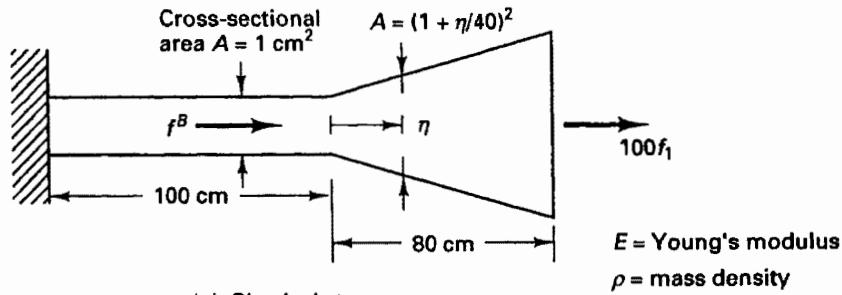
text_image

Cross-sectional area A = 1 cm² A = (1 + η/40)² f^B η 100 cm 100f₁ 80 cm E = Young's modulus ρ = mass density

(a) Physical structure 

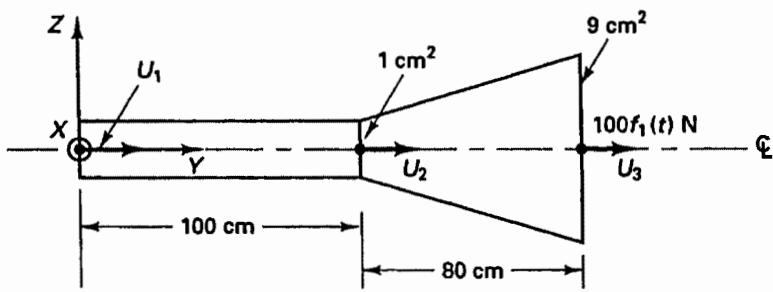
text_image

Z U₁ 1 cm² 9 cm² X Y U₂ 100 f₁(t) N U₃ 100 cm 80 cm C

(b) Element assemblage in global system 

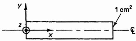
text_image

y z x 1 cm² ξ

(c) Element 1, $f_{x}^{B} = f_{2}(t)$ N/cm³ 

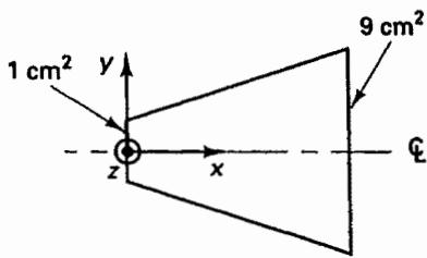
text_image

1 cm² y 9 cm² z x ξ

(d) Element 2, $f_{x}^{B} = 0.1 \ f_{2}(t) \ \mathrm{N/cm^{3}}$ 

line

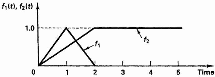
| Time | f₁(t) | f₂(t) | |------|-------|-------| | 0 | 0 | 0 | | 1 | 1.0 | 0.5 | | 2 | 0 | 1.0 | | 3 | 0 | 1.0 | | 4 | 0 | 1.0 | | 5 | 0 | 1.0 |

(e) Time variation of loads Figure E4.5 Two-element bar assemblage In the formulation of the finite element equilibrium equations we employ the general equations (4.8) to (4.24) but use that the only nonzero stress is the longitudinal stress in the bar. Furthermore, considering the complete bar as an assemblage of 2 two-node bar elements corresponds to assuming a linear displacement variation between the nodal points of each element. The first step is to construct the matrices $\mathbf{H}^{(m)}$ and $\mathbf{B}^{(m)}$ for m = 1, 2. We recall that although the displacement at the left end of the structure is zero, we first include the displacement at that surface in the construction of the finite element equilibrium equations. Corresponding to the displacement vector $U^{T} = [U_{1} \quad U_{2} \quad U_{3}]$ , we have $$ \mathbf {H} ^ {(1)} = \left[ \left(1 - \frac {x}{1 0 0}\right) \frac {x}{1 0 0} 0 \right] $$ $$ \mathbf {B} ^ {(1)} = \left[ - \frac {1}{1 0 0} \quad \frac {1}{1 0 0} \quad 0 \right] $$ $$ \mathbf {H} ^ {(2)} = \left[ 0 \quad \left(1 - \frac {x}{8 0}\right) \quad \frac {x}{8 0} \right] $$ $$ \mathbf {B} ^ {(2)} = \left[ \begin{array}{l l l} 0 & - \frac {1}{8 0} & \frac {1}{8 0} \end{array} \right] $$ The material property matrices are $$ \mathbf {C} ^ {(1)} = E; \quad \mathbf {C} ^ {(2)} = E $$ where E is Young's modulus for the material. For the volume integrations we need the cross-sectional areas of the elements. We have $$ A ^ {(1)} = 1 \mathrm{cm} ^ {2}; \quad A ^ {(2)} = \left(1 + \frac {x}{4 0}\right) ^ {2} \mathrm{cm} ^ {2} $$ When the loads are applied very slowly, a static analysis is required in which the stiffness matrix K and load vector R must be calculated. The body forces and loads are given in Fig. E4.5. We therefore have $$ \mathbf {K} = (1) E \int_ {0} ^ {1 0 0} \left[ \begin{array}{c} - \frac {1}{1 0 0} \\ \frac {1}{1 0 0} \\ 0 \end{array} \right] \left[ \begin{array}{l l l} - \frac {1}{1 0 0} & \frac {1}{1 0 0} & 0 \end{array} \right] d x + E \int_ {0} ^ {8 0} \left(1 + \frac {x}{4 0}\right) ^ {2} \left[ \begin{array}{c} 0 \\ - \frac {1}{8 0} \\ \frac {1}{8 0} \end{array} \right] \left[ \begin{array}{l l l} 0 & - \frac {1}{8 0} & \frac {1}{8 0} \end{array} \right] d x $$ $$ \mathbf {K} = \frac {E}{1 0 0} \left[ \begin{array}{r r r} 1 & - 1 & 0 \\ - 1 & 1 & 0 \\ 0 & 0 & 0 \end{array} \right] + \frac {1 3 E}{2 4 0} \left[ \begin{array}{r r r} 0 & 0 & 0 \\ 0 & 1 & - 1 \\ 0 & - 1 & 1 \end{array} \right] $$ $$ = \frac {E}{2 4 0} \left[ \begin{array}{r r r} 2. 4 & - 2. 4 & 0 \\ - 2. 4 & 1 5. 4 & - 1 3 \\ 0 & - 1 3 & 1 3 \end{array} \right] \tag {a} $$ and also, $$ \begin{array}{l} \mathbf {R} _ {B} = \left\{(1) \int_ {0} ^ {1 0 0} \left[ \begin{array}{c} 1 - \frac {x}{1 0 0} \\ \frac {x}{1 0 0} \\ 0 \end{array} \right] (1) d x + \int_ {0} ^ {8 0} \left(1 + \frac {x}{4 0}\right) ^ {2} \left[ \begin{array}{c} 0 \\ 1 - \frac {x}{8 0} \\ \frac {x}{8 0} \end{array} \right] \left(\frac {1}{1 0}\right) d x \right\} f _ {2} (t) \\ = \frac {1}{3} \left[ \begin{array}{l} 1 5 0 \\ 1 8 6 \\ 6 8 \end{array} \right] f _ {2} (t) \tag {b} \\ \end{array} $$ $$ \mathbf {R} _ {C} = \left[ \begin{array}{c} 0 \\ 0 \\ 1 0 0 \end{array} \right] f _ {1} (t) \tag {c} $$ To obtain the solution at a specific time $t^*$ , the vectors $\mathbf{R}_B$ and $\mathbf{R}_C$ must be evaluated corresponding to $t^*$ , and the equation $$ \mathbf {K U} \left| _ {t = t ^ {*}} = \mathbf {R} _ {B} \right| _ {t = t ^ {*}} + \mathbf {R} _ {C} \left| _ {t = t ^ {*}} \right. \tag {d} $$ yields the displacements at $t^{*}$ . We should note that in this static analysis the displacements at time $t^{*}$ depend only on the magnitude of the loads at that time and are independent of the loading history. Considering now the dynamic analysis, we also need to calculate the mass matrix. Using the displacement interpolations and (4.25), we have $$ \begin{array}{l} \mathbf {M} = (1) \rho \int_ {0} ^ {1 0 0} \left[ \begin{array}{c} 1 - \frac {x}{1 0 0} \\ \frac {x}{1 0 0} \\ 0 \end{array} \right] \left[ \left(1 - \frac {x}{1 0 0}\right) \quad \frac {x}{1 0 0} \quad 0 \right] d x \\ + \rho \int_ {0} ^ {8 0} \left(1 + \frac {x}{4 0}\right) ^ {2} \left[ \begin{array}{c} 0 \\ 1 - \frac {x}{8 0} \\ \frac {x}{8 0} \end{array} \right] \left[ \begin{array}{l l l} 0 & \left(1 - \frac {x}{8 0}\right) & \frac {x}{8 0} \end{array} \right] d x \\ \end{array} $$ Hence $\mathbf{M} = \frac{\rho}{6}\left[ \begin{array}{ccc}200 & 100 & 0\\ 100 & 584 & 336\\ 0 & 336 & 1024 \end{array} \right]$ Damping was not specified; thus, the equilibrium equations now to be solved are $$ \mathbf {M} \ddot {\mathbf {U}} (t) + \mathbf {K} \mathbf {U} (t) = \mathbf {R} _ {B} (t) + \mathbf {R} _ {C} (t) \tag {e} $$ where the stiffness matrix $\mathbf{K}$ and load vectors $\mathbf{R}_B$ and $\mathbf{R}_C$ have already been given in (a) to (c). Using the initial conditions $$ \mathbf {U} \mid_ {t = 0} = \mathbf {0}; \quad \dot {\mathbf {U}} \mid_ {t = 0} = \mathbf {0} \tag {f} $$ these dynamic equilibrium equations must be integrated from time 0 to time $t^{*}$ in order to obtain the solution at time $t^{*}$ (see Chapter 9). To actually solve for the response of the structure in Fig. E4.5(a), we need to impose $U_{1}=0$ for all time t. Hence, the equations (d) and (e) must be amended by this condition (see Section 4.2.2). The solution of (d) and (e) then yields $U_{2}(t)$ , $U_{3}(t)$ , and the stresses are obtained using $$ \tau_ {x x} ^ {(m)} = \mathbf {C} ^ {(m)} \mathbf {B} ^ {(m)} \mathbf {U} (t); \quad m = 1, 2 \tag {g} $$ These stresses will be discontinuous between the elements because constant element strains are assumed. Of course, in this example, since the exact solution to the mathematical model can be computed, stresses more accurate than those given by (g) could be evaluated within each element. In static analysis, this increase in accuracy could simply be achieved, as in beam theory, by adding a stress correction for the distributed element loading to the values given in (g). However, such a stress correction is not straightforward in general dynamic analysis (and in any two- and three-dimensional practical analysis), and if a large number of elements is used to represent the structure, the stresses using (g) are sufficiently accurate (see Section 4.3.6). EXAMPLE 4.6: Consider the analysis of the cantilever plate shown in Fig. E4.6. To illustrate the analysis technique, use the coarse finite element idealization given in the figure (in a practical analysis more finite elements must be employed (see Section 4.3). Establish the matrices $\mathbf{H}^{(2)}$ , $\mathbf{B}^{(2)}$ , and $\mathbf{C}^{(2)}$ . The cantilever plate is acting in plane stress conditions. For an isotropic linear elastic material the stress-strain matrix is defined using Young's modulus E and Poisson's ratio $\nu$ (see Table 4.3), $$ \mathbf {C} ^ {(2)} = \frac {E}{1 - \nu^ {2}} \left[ \begin{array}{c c c} 1 & \nu & 0 \\ \nu & 1 & 0 \\ 0 & 0 & \frac {1 - \nu}{2} \end{array} \right] $$ The displacement transformation matrix $\mathbf{H}^{(2)}$ of element 2 relates the element internal displacements to the nodal point displacements, $$ \left[ \begin{array}{l} u (x, y) \\ v (x, y) \end{array} \right] ^ {(2)} = \mathbf {H} ^ {(2)} \mathbf {U} \tag {a} $$ where U is a vector listing all nodal point displacements of the structure, $$ \mathbf {U} ^ {T} = \left[ \begin{array}{l l l l l l l} U _ {1} & U _ {2} & U _ {3} & U _ {4} & \dots & U _ {1 7} & U _ {1 8} \end{array} \right] \tag {b} $$ (As mentioned previously, in this phase of analysis we are considering the structural model without displacement boundary conditions.) In considering element 2, we recognize that only the displacements at nodes 6, 3, 2, and 5 affect the displacements in the element. For computational purposes it is convenient to use a convention to number the element nodal points and corresponding element degrees of freedom as shown in Fig E4.6(c). In the same figure the global structure degrees of freedom of the vector U in (b) are also given. To derive the matrix $\mathbf{H}^{(2)}$ in (a) we recognize that there are four nodal point displacements each for expressing $u(x, y)$ and $v(x, y)$ . Hence, we can assume that the local element displacements u and v are given in the following form of polynomials in the local coordinate variables x and y: $$ u (x, y) = \alpha_ {1} + \alpha_ {2} x + \alpha_ {3} y + \alpha_ {4} x y \tag {c} $$ $$ v (x, y) = \beta_ {1} + \beta_ {2} x + \beta_ {3} y + \beta_ {4} x y $$ 

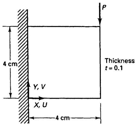
text_image

4 cm Y, V X, U 4 cm Thickness t = 0.1 P

(a) Cantilever plate 

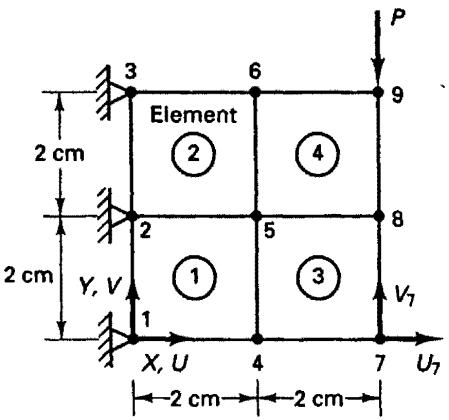
text_image

Element 2 cm 2 cm Y, V 1 X, U 4 6 9 5 3 2 cm 2 cm 7 U7 P V7

(b) Finite element idealization (plane stress condition) 

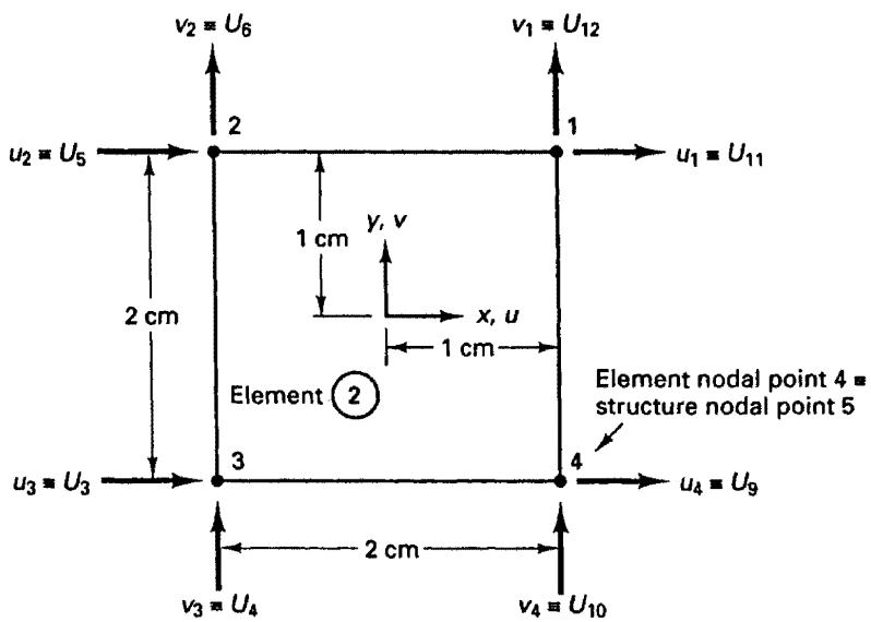
text_image

v2 = U6 v1 = U12 u2 = U5 2 1 u1 = U11 2 cm 1 cm y, v x, u 1 cm Element ② Element nodal point 4 = structure nodal point 5 u3 = U3 3 4 u4 = U9 2 cm v3 = U4 v4 = U10

(c) Typical two-dimensional four-node element defined in local coordinate system Figure E4.6 Finite element plane stress analysis The unknown coefficients $\alpha_{1},\ldots ,\beta_{4}$ , which are also called the generalized coordinates, will be expressed in terms of the unknown element nodal point displacements $u_{1},\ldots ,u_{4}$ and $v_{1},\ldots ,v_{4}$ . Defining $$ \hat {\mathbf {u}} ^ {T} = \left[ \begin{array}{l l l l l l l l l} u _ {1} & u _ {2} & u _ {3} & u _ {4} & v _ {1} & v _ {2} & v _ {3} & v _ {4} \end{array} \right] \tag {d} $$ we can write (c) in matrix form: $$ \left[ \begin{array}{l} u (x, y) \\ v (x, y) \end{array} \right] = \boldsymbol {\Phi} \boldsymbol {\alpha} \tag {e} $$ where $\Phi = \begin{bmatrix} \phi & 0 \\ 0 & \phi \end{bmatrix}; \quad \phi = [1 \quad x \quad y \quad xy]$ and $\mathbf{a}\mathbf{a}^T = [\alpha_1\alpha_2\alpha_3\alpha_4\beta_1\beta_2\beta_3\beta_4]$ Equation (e) must hold for all nodal points of the element; therefore, using (d), we have $$ \hat {\mathbf {u}} = \mathbf {A} \boldsymbol {\alpha} \tag {f} $$ in which $\mathbf{A} = \begin{bmatrix} \mathbf{A}_1 & \mathbf{0} \\ \mathbf{0} & \mathbf{A}_1 \end{bmatrix}$ and $\mathbf{A}_1 = \begin{bmatrix} 1 & 1 & 1 & 1 \\ 1 & -1 & 1 & -1 \\ 1 & -1 & -1 & 1 \\ 1 & 1 & -1 & -1 \end{bmatrix}$ Solving from (f) for $\alpha$ and substituting into (e), we obtain $$ \mathbf {H} = \boldsymbol {\Phi} \mathbf {A} ^ {- 1} \tag {g} $$ where the fact that no superscript is used on H indicates that the displacement interpolation matrix is defined corresponding to the element nodal point displacements in (d), $$ \mathbf {H} = \frac {1}{4} \left[ \begin{array}{c c c c} (1 + x) (1 + y) & (1 - x) (1 + y) & (1 - x) (1 - y) & (1 + x) (1 - y) \\ 0 & 0 & 0 & 0 \\ 0 & 0 & 0 & 0 \\ (1 + x) (1 + y) & (1 - x) (1 + y) & (1 - x) (1 - y) & (1 + x) (1 - y) \end{array} \right] \tag {h} $$ The displacement functions in H could also have been established by inspection. Let $H_{ij}$ be the $(i,j)$ th element of H; then $H_{11}$ corresponds to a function that varies linearly in x and y [as required in (c)], is unity at x = 1, y = 1, and is zero at the other three element nodes. We discuss the construction of the displacement functions in H based on these thoughts in Section 5.2. With $\mathbf{H}$ given in (h) we have $$ \mathbf {H} ^ {(2)} = \left[ \begin{array}{c c c c c c c c c c c} 0 & 0 & 0 & 0 & 0 & 0 & 0 & 0 & 0 & 0 & 0 \\ 0 & 0 & 0 & 0 & 0 & 0 & 0 & 0 & 0 & 0 & 0 \\ 0 & 0 & 0 & 0 & 0 & 0 & 0 & 0 & 0 & 0 & 0 \\ 0 & 0 & 0 & 0 & 0 & 0 & 0 & 0 & 0 & 0 & 0 \\ H _ {1 3} & H _ {1 7} & H _ {1 2} & H _ {1 6} & 0 & 0 & H _ {1 4} & H _ {1 8} & 0 & 0 & 0 \\ H _ {2 3} & H _ {2 7} & H _ {2 2} & H _ {2 6} & 0 & 0 & H _ {2 4} & H _ {2 8} & 0 & 0 & 0 \\ 0 & 0 & 0 & 0 & 0 & 0 & 0 & 0 & 0 & 0 & 0 \\ 0 & 0 & 0 & 0 & 0 & 0 & 0 & 0 & 0 & 0 & 0 \\ 0 & 0 & 0 & 0 & 0 & 0 & 0 & 0 \\ 0 & 0 & 0 & 0 & 0 & 0 & 0 & 0 & 0 & 0 & 0 \\ 0 & 0 & 0 & 0 & 0 & 0 & 0 & 0 & 0 & 0 & 0 \\ 0 & 0 & 0 & \text { } & 0 & 0 & 0 & 0 & 0 & 0 & 0 \\ 0 & 0 & 0 & 0 & 0 & 0 & 0 & 0 & 0 & 0 & 0 \\ 0 & 0 & 0 & 0 & 0 & 0 & 0 & 0 & 0 & 0 & 0 \\ 0 & 0 & 0 & 0. 5 & 0 & 0 & 0 & 0 & 0 & 0 & 0 \\ 0 & 0 & 0 & 0 & 0 & 0 & 0 & 0 & 0 & 0 & 0 \\ 0 & 0 & 0 & 0 & 0 & 0 & 0 & 0 & 0 & 0 & 0 \\ 0 & 0 & 0 & 0, 0 & 0 & 0 & 0 & 0 & 0 & 0 & 0 \\ 0 & 0 & 0 & 0 & 0 & 0 & 0 & 0 & 0 & 0 & 0 \\ 0 & 0 & 0 & 0 & 0 & 0 & 0 & 0 & 0 & 0 & 0 \\ 0 & 0 & 0 & H _ {1 3} & H _ {1 7} & H _ {1 2} & H _ {1 6} & 0 & 0 & 0 & 0 \\ 0 & 0 & 0 & 0 & 0 & 0 & 0 & 0 & 0 & 0 & 0 \\ 0 & 0 & 0 & 0 & 0 & 0 & 0 & 0 & 0 & 0 & 0 \\ 0 & 0 & 0 & 0 & 0 & 0 & 0. 5 & 0 & 0 & 0 & 0 \\ 0 & 0 & 0 & 0 & 0 & 0 & 0 & 0 & 0 & 0 & 0 \\ 0 & 0 & 0 & 0 & 0 & 0 & 0 & 0 & 0 & 0 & 0 \\ 0 & 0 & 0 & 0 & 0 & 0 & 0, 0 & 0 & 0 & 0 & 0 \\ 0 & 0 & 0 & 0 & 0 & 0 & 0 & 0 & 0 & 0 & 0 \\ 0 & 0 & 0 & 0 & 0 & 0 & 0 & 0 & 0 & 0 & 0 \\ 0 & 0 & 0 & 0 & 0 & 0 & \text { } & 0 & 0 & 0 & 0 \\ 0 & 0 & 0 & 0 & 0 & 0 & 0 & 0 & 0 & 0 & 0 \\ 0 & 0 & 0 & 0 & 0 & 0 & 0 & 0 & 0 & 0 & 0 \\ 0 & 0 & 0 & 0 & 0 & 0 & 0 \\ 0 & 0 & 0 & 0 & 0 & 0 & 0 & 0 & 0 & 0 & 0 \\ 0 & 0 & 0 & 0 & 0 & 0 & 0 & 0 & 0 & 0 & 0 \\ 0 & 0 & 0 & 0 & \text { } & 0 & 0 & 0 & 0 & 0 & 0 \\ 0 & 0 & 0 & 0 & 0 & 0 & 0 & 0 & 0 & 0 & 0 \\ 0 & 0 & 0 & 0 & 0 & 0 & 0 & 0 & 0 & 0 & 0 \\ 0 & 0 & 0 & 0 & 0, 0 & 0 & 0 & 0 & 0 & 0 & 0 \\ 0 & 0 & 0 & 0 & 0 & 0 & 0 & 0 & 0 & 0 & 0 \\ 0 & 0 & 0 & 0 & 0 & 0 & 0 & 0 & 0 & 0 & 0 \\ 0 & 0 & 0 & 0 & H _ {1 3} & H _ {1 7} & H _ {1 2} & H _ {1 6} & 0 & 0 & 0 \\ 0 & 0 & 0 & 0 & 0 & 0 & 0 & 0 & 0 & 0 & 0 \\ 0 & 0 & 0 & 0 & 0 & 0 & 0 & 0 & 0 & 0 & 0 \\ 0 & 0 & 0 & 0 & 0 & 0 & 0 & 1 3 & 0 & 0 & 0 \\ 0 & 0 & 0 & 0 & 0 & 0 & 0 & 0 & 0 & 0 & 0 \\ 0 & 0 & 0 & 0 & 0 & 0 & 0 & 0 & 0 & 0 & 0 \\ 0 & 0 & 0 & 0 & 0 & 0 & 0 & 0, 0 & 0 & 0 & 0 \\ 0 & 0 & 0 & 0 & 0 & 0 & 0 & 0 & 0 & 0 & 0 \\ 0 & 0 & 0 & 0 & 0 & 0 & 0 & 0 & 0 & 0 & 0 \\ 0 & 0 & 0 & 0 & 0 & 0 & 0 & \text { } & 0 & 0 & 0 \\ 0 & 0 & 0 & 0 & 0 & 0 & 0 & 0 & 0 & 0 & 0 \\ 0 & 0 & 0 & 0 & 0 & 0 & 0 & 0 & 0 & 0 & 0 \\ 0 & 0 & 0 & 0 & 0 & 0 & 0 & 0. 5 & 0 & 0 & 0 \\ 0 & 0 & 0 & 0 & 0 & 0 & 0 & 0 & 0 & 0 & 0 \\ 0 & 0 & 0 & 0 & 0 & 0 & 0 & 0 & 0 & 0 & 0 \\ 0 & 0 & 0 & 0 & 0 & 0 & 0 & 0 | & 0 & 0 & 0 \\ 0 & 0 & 0 & 0 & 0 & 0 & 0 & 0 | & 0 & 0 & 0 \\ 0 & 0 & 0 & 0 & 0 & 0 & 0 & 0 | & 0 & 0 & 0 \\ 0 & 0 & 0 & 0 & 0 & 0 & 0 & \text { } & 0 & 0 & 0 \\ 0 & 0 & 0 & 0 & 0 & 0 & 0 & 0 | & 0 & 0 & 0 \\ 0 & 0 & 0 & 0 & 0 & 0 & 0 & 0 | & 0 & 0 & 0 \\ 0 & 0 & 0 & 0 & 0 & 0 & 0 & H _ {1 4} & H _ {1 8} & 0 & 0 \\ 0 & 0 & 0 & 0 & 0 & 0 & 0 & 0 | & 0 & 0 & 0 \\ 0 & 0 & 0 & 0 & 0 & 0 & 0 & 0 | & 0 & 0 & 0 \\ 0 & 0 & 0 & 0 & 0 & 0 & 0 & 0 | \\ 0 & 0 & 0 & 0 & 0 & 0 & 0 & 0 | & 0 & 0 & 0 \\ 0 & 0 & 0 & 0 & 0 & 0 & 0 & 0 | & 0 & 0 & 0 \\ 0 & 0 & 0 & 0 & 0 & 0 & 0 & 0 | & 0 & 0 \\ 0 & 0 & 0 & 0 & 0 & 0 & 0 & 0 | & 0 & 0 & 0 \\ 0 & 0 & 0 & 0 & 0 & 0 & 0 & 0 | & 0 & 0 & 0 \\ 0 & 0 & 0 & 0 & 0 & 0 & 0 & 0 | \end{array} \right] $$ $$ \begin{array}{c c c c c} u _ {1} & v _ {1} \leftarrow \text { Element degrees of freedom } \\ U _ {1 1} & U _ {1 2} & U _ {1 3} & U _ {1 4} & U _ {1 8} \leftarrow \text { Assemblage degrees } \\ \left[ \begin{array}{c c c c c} H _ {1 1} & H _ {1 5} & 0 & 0 & \dots \text { zeros } \dots 0 \\ H _ {2 1} & H _ {2 5} & 0 & 0 & \dots \text { zeros } \dots 0 \end{array} \right] & \text { of freedom } \end{array} \tag {i} $$ The strain-displacement matrix can now directly be obtained from (g). In plane stress conditions the element strains are $$ \epsilon^ {T} = \left[ \begin{array}{c c c} \epsilon_ {x x} & \epsilon_ {y y} & \gamma_ {x y} \end{array} \right] $$ where $\epsilon_{xx} = \frac{\partial u}{\partial x};\qquad \epsilon_{yy} = \frac{\partial v}{\partial y};\qquad \gamma_{xy} = \frac{\partial u}{\partial y} +\frac{\partial v}{\partial x}$ Using (g) and recognizing that the elements in $\mathbf{A}^{-1}$ are independent of $x$ and $y$ , we obtain $$ \mathbf {B} = \mathbf {E A} ^ {- 1} $$ where $\mathbf{E} = \begin{bmatrix} 0 & 1 & 0 & y & 0 & 0 & 0 & 0 \\ 0 & 0 & 0 & 0 & 0 & 0 & 1 & x \\ 0 & 0 & 1 & x & 0 & 1 & 0 & y \end{bmatrix}$ Hence, the strain-displacement matrix corresponding to the local element degrees of freedom is $$ \mathbf {B} = \frac {1}{4} \left[ \begin{array}{c c c c} (1 + y) & - (1 + y) & - (1 - y) & (1 - y) \\ 0 & 0 & 0 & 0 \\ (1 + x) & (1 - x) & - (1 - x) & - (1 + x) \end{array} \right. $$ $$ \left. \begin{array}{c c c c} 0 & 0 & 0 & 0 \\ (1 + x) & (1 - x) & - (1 - x) & - (1 + x) \\ (1 + y) & - (1 + y) & - (1 - y) & (1 - y) \end{array} \right] \tag {j} $$ The matrix $\mathbf{B}$ could also have been calculated directly by operating on the rows of the matrix $\mathbf{H}$ in (h). Let $B_{ij}$ be the $(i,j)$ th element of B; then we now have $$ \mathbf {B} ^ {(2)} = \left[ \begin{array}{c c c c c c c c c c c c c c c c} 0 & 0 & B _ {1 3} & B _ {1 7} & B _ {1 2} & B _ {1 6} & 0 & 0 & B _ {1 4} & B _ {1 8} & B _ {1 1} & B _ {1 5} & 0 & 0 \\ 0 & 0 & B _ {2 3} & B _ {2 7} & B _ {2 2} & B _ {2 6} & 0 & 0 & B _ {2 4} & B _ {2 8} & B _ {2 1} & B _ {2 5} & 0 & 0 \\ 0 & 0 & B _ {3 3} & B _ {3 7} & B _ {3 2} & B _ {3 6} & 0 & 0 & B _ {3 4} & B _ {3 8} & B _ {3 1} & B _ {3 5} & 0 & 0 \end{array} \right] $$ $$ \left. \begin{array}{c} 0 \\ \dots \text {zeroes} \dots 0 \\ 0 \end{array} \right] $$ where the element degrees of freedom and assemblage degrees of freedom are ordered as in (d) and (b). EXAMPLE 4.7: A linearly varying surface pressure distribution as shown in Fig. E4.7 is applied to element (m) of an element assemblage. Evaluate the vector $\mathbf{R}_{s}^{(m)}$ for this element. The first step in the calculation of $\mathbf{R}_{s}^{(m)}$ is the evaluation of the matrix $\mathbf{H}^{S(m)}$ . This matrix can be established using the same approach as in Example 4.6. For the surface displacements we assume $$ u ^ {S} = \alpha_ {1} + \alpha_ {2} x + \alpha_ {3} x ^ {2} $$ $$ v ^ {s} = \beta_ {1} + \beta_ {2} x + \beta_ {3} x ^ {2} \tag {a} $$ where (as in Example 4.6) the unknown coefficients $\alpha_{1},\ldots ,\beta_{3}$ are evaluated using the nodal point displacements. We thus obtain $$ \left[ \begin{array}{l} u ^ {s} (x) \\ v ^ {s} (x) \end{array} \right] = \mathbf {H} ^ {s} \hat {\mathbf {u}} $$ $$ \hat {\mathbf {u}} ^ {T} = \left[ \begin{array}{l l l l l l l} u _ {1} & u _ {2} & u _ {3} & v _ {1} & v _ {2} & v _ {3} \end{array} \right] $$ and $$ \mathbf {H} ^ {s} = \left[ \begin{array}{c c c c c c} \frac {1}{2} x (1 + x) & - \frac {1}{2} x (1 - x) & (1 - x ^ {2}) & 0 & 0 & 0 \\ 0 & 0 & 0 & \frac {1}{2} x (1 + x) & - \frac {1}{2} x (1 - x) & (1 - x ^ {2}) \end{array} \right] $$