Using the relations (4.33) to (4.37), we thus have $$ \begin{array}{l} \mathbf {K} = \mathbf {A} ^ {- T} \left\{\int_ {A} \frac {E (1 - \nu)}{(1 + \nu) (1 - 2 \nu)} \left[ \begin{array}{l l l l} 0 & 0 & 0 & \frac {1}{x} \\ 1 & 0 & 0 & 1 \\ 0 & 0 & 1 & \frac {y}{x} \\ 0 & 0 & 0 & 0 \\ 0 & 0 & 1 & 0 \\ 0 & 1 & 0 & 0 \end{array} \right] \left[ \begin{array}{c c c c} 1 & \frac {\nu}{1 - \nu} & 0 & \frac {\nu}{1 - \nu} \\ \frac {\nu}{1 - \nu} & 1 & 0 & \frac {\nu}{1 - \nu} \\ 0 & 0 & \frac {1 - 2 \nu}{2 (1 - \nu)} & 0 \\ \frac {\nu}{1 - \nu} & \frac {\nu}{1 - \nu} & 0 & 1 \end{array} \right] \right. \\ \left[ \begin{array}{c c c c c c} 0 & 1 & 0 & 0 & 0 & 0 \\ 0 & 0 & 0 & 0 & 0 & 1 \\ 0 & 0 & 1 & 0 & 1 & 0 \\ \frac {1}{x} & 1 & \frac {y}{x} & 0 & 0 & 0 \end{array} \right] x d x d y \Bigg \} \mathbf {A} ^ {- 1} \quad (\mathrm{a}) \\ \end{array} $$ where 1 radian of the axisymmetric element is considered in the volume integration. Similarly, we have $$ \mathbf {R} _ {B} = \mathbf {A} ^ {- T} \int_ {A} \left[ \begin{array}{l l} 1 & 0 \\ x & 0 \\ y & 0 \\ 0 & 1 \\ 0 & x \\ 0 & y \end{array} \right] \left[ \begin{array}{l} f _ {x} ^ {B} \\ f _ {y} ^ {B} \end{array} \right] x d x d y $$ $$ \mathbf {R} _ {I} = \mathbf {A} ^ {- T} \int_ {A} \left[ \begin{array}{l l l l} 0 & 0 & 0 & \frac {1}{x} \\ 1 & 0 & 0 & 1 \\ 0 & 0 & 1 & \frac {y}{x} \\ 0 & 0 & 0 & 0 \\ 0 & 0 & 1 & 0 \\ 0 & 1 & 0 & 0 \end{array} \right] \left[ \begin{array}{l} \tau_ {x x} ^ {I} \\ \tau_ {y y} ^ {I} \\ \tau_ {x y} ^ {I} \\ \tau_ {z z} ^ {I} \end{array} \right] x d x d y \tag {b} $$ $$ \mathbf {M} = \rho \mathbf {A} ^ {- T} \left\{\int_ {A} \left[ \begin{array}{l l} 1 & 0 \\ x & 0 \\ y & 0 \\ 0 & 1 \\ 0 & x \\ 0 & y \end{array} \right] \left[ \begin{array}{l l l l l l} 1 & x & y & 0 & 0 & 0 \\ 0 & 0 & 0 & 1 & x & y \end{array} \right] x d x d y \right\} \mathbf {A} ^ {- 1} $$ where the mass density $\rho$ is assumed to be constant. For calculation of the surface load vector $R_{s}$ , it is expedient in practice to introduce auxiliary coordinate systems located along the loaded sides of the element. Assume that the side 2–3 of the element is loaded as shown in Fig. E4.17. The load vector $R_{s}$ is then evaluated using as the variable s, $$ \mathbf {R} _ {s} = \int_ {s} \left[ \begin{array}{c c} 0 & 0 \\ 1 - \frac {s}{L} & 0 \\ \frac {s}{L} & 0 \\ 0 & 0 \\ 0 & 1 - \frac {s}{L} \\ 0 & \frac {s}{L} \end{array} \right] \left[ \begin{array}{l} f _ {x} ^ {s} \\ f _ {y} ^ {s} \end{array} \right] \left[ \begin{array}{l} x _ {2} \left(1 - \frac {s}{L}\right) + x _ {3} \frac {s}{L} \end{array} \right] d s $$ Considering these finite element matrix evaluations the following observations can be made. First, to evaluate the integrals, it is possible to obtain closed-form solutions; alternatively, numerical integration (discussed in Section 5.5) can be used. Second, we find that the stiffness, mass, and load matrices corresponding to plane stress and plane strain finite elements can be obtained simply by (1) not including the fourth row in the strain-displacement matrix E used in (a) and (b), (2) employing the appropriate stress-strain matrix C in (a), and (3) using as the differential volume element h dx dy instead of x dx dy, where h is the thickness of the element (conveniently taken equal to 1 in plane strain analysis). Therefore, axisymmetric, plane stress, and plane strain analyses can effectively be implemented in a single computer program. Also, the matrix E shows that constant-strain conditions $\epsilon_{xx}$ , $\epsilon_{yy}$ , and $\gamma_{xy}$ are assumed in either analysis. The concept of performing axisymmetric, plane strain, and plane stress analysis in an effective manner in one computer program is, in fact, presented in Section 5.6, where we discuss the efficient implementation of isoparametric finite element analysis. 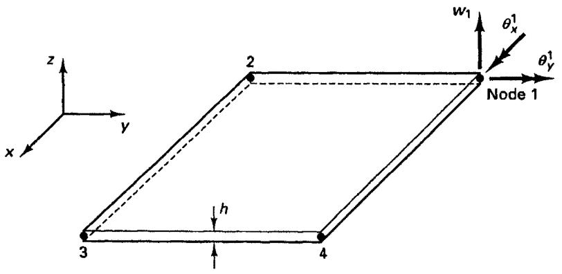EXAMPLE 4.18: Derive the matrices $\Phi(x, y)$ , $\mathbf{E}(x, y)$ , and $\mathbf{A}$ for the rectangular plate bending element in Fig. E4.18. This element is one of the first plate bending elements derived, and more effective plate bending elements are already in use (see Section 5.4.2). As shown in Fig. E4.18, the plate bending element considered has three degrees of freedom per node. Therefore, it is necessary to have 12 unknown generalized coordinates, $\alpha_{1}, \ldots, \alpha_{12}$ , 

text_image

z x y 2 w₁ θₓ¹ θᵧ¹ Node 1 3 4 h

Figure E4.18 Rectangular plate bending element. in the displacement assumption for $w$ . The polynomial used is $$ \begin{array}{l} w = \alpha_ {1} + \alpha_ {2} x + \alpha_ {3} y + \alpha_ {4} x ^ {2} + \alpha_ {5} x y + \alpha_ {6} y ^ {2} + \alpha_ {7} x ^ {3} + \alpha_ {8} x ^ {2} y \\ + \alpha_ {9} x y ^ {2} + \alpha_ {1 0} y ^ {3} + \alpha_ {1 1} x ^ {3} y + \alpha_ {1 2} x y ^ {3} \\ \end{array} $$ Hence, $$ \phi (x, y) = \left[ \begin{array}{l l l l l l l l l l l l} 1 & x & y & x ^ {2} & x y & y ^ {2} & x ^ {3} & x ^ {2} y & x y ^ {2} & y ^ {3} & x ^ {3} y & x y ^ {3} \end{array} \right] \tag {a} $$ We can now calculate $\partial w / \partial x$ and $\partial w / \partial y$ : $$ \frac {\partial w}{\partial x} = \alpha_ {2} + 2 \alpha_ {4} x + \alpha_ {5} y + 3 \alpha_ {7} x ^ {2} + 2 \alpha_ {8} x y + \alpha_ {9} y ^ {2} + 3 \alpha_ {1 1} x ^ {2} y + \alpha_ {1 2} y ^ {3} \tag {b} $$ and $$ \frac {\partial w}{\partial y} = \alpha_ {3} + \alpha_ {5} x + 2 \alpha_ {6} y + \alpha_ {8} x ^ {2} + 2 \alpha_ {9} x y + 3 \alpha_ {1 0} y ^ {2} + \alpha_ {1 1} x ^ {3} + 3 \alpha_ {1 2} x y ^ {2} \tag {c} $$ Using the conditions $$ \left. \begin{array}{l} w _ {i} = (w) _ {x _ {i}, y _ {i}}; \quad \theta_ {x} ^ {i} = \left(\frac {\partial w}{\partial y}\right) _ {x _ {i}, y _ {i}} \\ \theta_ {y} ^ {i} = \left(- \frac {\partial w}{\partial x}\right) _ {x _ {i}, y _ {i}} \end{array} \right\} i = 1, \dots , 4 $$ we can construct the matrix A, obtaining $$ \left[ \begin{array}{c} w _ {1} \\ \vdots \\ w _ {4} \\ \theta_ {x} ^ {1} \\ \vdots \\ \dot {\theta} _ {x} ^ {4} \\ \theta_ {y} ^ {1} \\ \vdots \\ \dot {\theta} _ {y} ^ {4} \end{array} \right] = \mathbf {A} \left[ \begin{array}{c} \alpha_ {1} \\ \alpha_ {2} \\ \vdots \\ \vdots \\ \alpha_ {1 2} \end{array} \right] $$ where $$ \mathbf {A} = \left[ \begin{array}{c c c c c c c c c c c c} 1 & x _ {1} & y _ {1} & x _ {1} ^ {2} & x _ {1} y _ {1} & y _ {1} ^ {2} & x _ {1} ^ {3} & x _ {1} ^ {2} y _ {1} & x _ {1} y _ {1} ^ {2} & y _ {1} ^ {3} & x _ {1} ^ {3} y _ {1} & x _ {1} y _ {1} ^ {3} \\ \vdots & & & & \vdots & & & & & & & \\ 1 & x _ {4} & y _ {4} & x _ {4} ^ {2} & x _ {4} y _ {4} & y _ {4} ^ {2} & x _ {4} ^ {3} & x _ {4} ^ {2} y _ {4} & x _ {4} y _ {4} ^ {2} & y _ {4} ^ {3} & x _ {4} ^ {3} y _ {4} & x _ {4} y _ {4} ^ {3} \\ 0 & 0 & 1 & 0 & x _ {1} & 2 y _ {1} & 0 & x _ {1} ^ {2} & 2 x _ {1} y _ {1} & 3 y _ {1} ^ {2} & x _ {1} ^ {3} & 3 x _ {1} y _ {1} ^ {2} \\ \vdots & & & & \vdots & & & & & & & \\ 0 & 0 & 1 & 0 & x _ {4} & 2 y _ {4} & 0 & x _ {4} ^ {2} & 2 x _ {4} y _ {4} & 3 y _ {4} ^ {2} & x _ {4} ^ {3} & 3 x _ {4} y _ {4} ^ {2} \\ 0 & - 1 & 0 & - 2 x _ {1} & - y _ {1} & 0 & - 3 x _ {1} ^ {2} & - 2 x _ {1} y _ {1} & - y _ {1} ^ {2} & 0 & - 3 x _ {1} ^ {2} y _ {1} & - y _ {1} ^ {3} \\ \vdots & & & & \vdots & & & & & & & \\ 0 & - 1 & 0 & - 2 x _ {4} & - y _ {4} & 0 & - 3 x _ {4} ^ {2} & - 2 x _ {4} y _ {4} & - y _ {4} ^ {2} & 0 & - 3 x _ {4} ^ {2} y _ {4} & - y _ {4} ^ {3} \end{array} \right] \tag {d} $$ which can be shown to be always nonsingular. To evaluate the matrix E, we recall that in plate bending analysis curvatures and moments are used as generalized strains and stresses (see Tables 4.2 and 4.3). Calculating the required derivatives of (b) and (c), we obtain $$ \frac {\partial^ {2} w}{\partial x ^ {2}} = 2 \alpha_ {4} + 6 \alpha_ {7} x + 2 \alpha_ {8} y + 6 \alpha_ {1 1} x y $$ $$ \frac {\partial^ {2} w}{\partial y ^ {2}} = 2 \alpha_ {6} + 2 \alpha_ {9} x + 6 \alpha_ {1 0} y + 6 \alpha_ {1 2} x y \tag {e} $$ $$ 2 \frac {\partial^ {2} w}{\partial x \partial y} = 2 \alpha_ {5} + 4 \alpha_ {8} x + 4 \alpha_ {9} y + 6 \alpha_ {1 1} x ^ {2} + 6 \alpha_ {1 2} y ^ {2} $$ Hence we have $$ \mathbf {E} = \left[ \begin{array}{c c c c c c c c c c c c c} 0 & 0 & 0 & 2 & 0 & 0 & 6 x & 2 y & 0 & 0 & 6 x y & 0 \\ 0 & 0 & 0 & 0 & 0 & 2 & 0 & 0 & 2 x & 6 y & 0 & 6 x y \\ 0 & 0 & 0 & 0 & 2 & 0 & 0 & 4 x & 4 y & 0 & 6 x ^ {2} & 6 y ^ {2} \end{array} \right] \tag {f} $$ With the matrices $\Phi$ , A, and E given in (a), (d), and (f) and the material matrix C in Table 4.3, the element stiffness matrix, mass matrix, and load vectors can now be calculated. An important consideration in the evaluation of an element stiffness matrix is whether the element is complete and compatible. The element considered in this example is complete as shown in (e) (i.e., the element can represent constant curvature states), but the element is not compatible. The compatibility requirements are violated in a number of plate bending elements, meaning that convergence in the analysis is in general not monotonic (see Section 4.3). 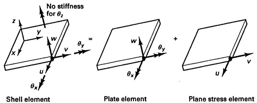EXAMPLE 4.19: Discuss the evaluation of the stiffness matrix of a flat rectangular shell element. A simple rectangular flat shell element can be obtained by superimposing the plate bending behavior considered in Example 4.18 and the plane stress behavior of the element used in Example 4.6. The resulting element is shown in Fig. E4.19. The element can be employed to model assemblages of flat plates (e.g., folded plate structures) and also curved shells. For actual analyses more effective shell elements are available, and we discuss here only the element in Fig. E4.19 in order to demonstrate some basic analysis approaches. Let $\mathbf{K}_B$ and $\mathbf{K}_M$ be the stiffness matrices, in the local coordinate system, corresponding to the bending and membrane behavior of the element, respectively. Then the shell element stiffness matrix $\tilde{\mathbf{K}}_S$ is $$ \tilde {\mathbf {K}} _ {S} = \left[ \begin{array}{c c} \tilde {\mathbf {K}} _ {B} & \mathbf {0} \\ 1 2 \times 1 2 & \\ \mathbf {0} & \tilde {\mathbf {K}} _ {M} \\ & 8 \times 8 \end{array} \right] \tag {a} $$ The matrices $\tilde{K}_{M}$ and $\tilde{K}_{B}$ were discussed in Examples 4.6 and 4.18, respectively. 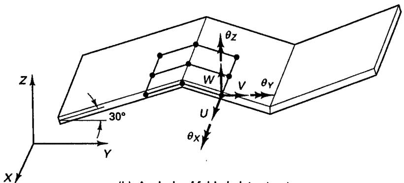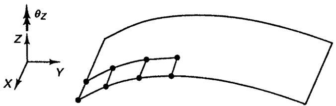This shell element can now be directly employed in the analysis of a variety of shell structures. Consider the structures in Fig. E4.19, which might be idealized as shown. Since we deal in these analyses with six degrees of freedom per node, the element stiffness matrices corresponding to the global degrees of freedom are calculated using the transformation given in (4.41) $$ \mathbf {K} _ {S} = \mathbf {T} ^ {T} \tilde {\mathbf {K}} _ {S} ^ {*} \mathbf {T} \tag {b} $$ where $\tilde{K}_{24\times24}^{*}=\begin{bmatrix}\tilde{K}_{20\times20}&0\\0&0\end{bmatrix}$ (c)  (a) Basic shell element with local five degrees of freedom at a node 

text_image

(b) Analysis of folded plate structure

(b) Analysis of folded plate structure 

text_image

θz z Y X

(c) Analysis of slightly curved shell Figure E4.19 Use of a flat shell element and $\mathbf{T}$ is the transformation matrix between the local and global element degrees of freedom. To define $\tilde{\mathbf{K}}_s^*$ corresponding to six degrees of freedom per node, we have amended $\tilde{\mathbf{K}}_s$ on the right-hand side of (c) to include the stiffness coefficients corresponding to the local rotations $\theta_z$ (rotations about the $z$ -axis) at the nodes. These stiffness coefficients have been set equal to zero in (c). The reason for doing so is that these degrees of freedom have not been included in the formulation of the element; thus the element rotation $\theta_z$ at a node is not measured and does not contribute to the strain energy stored in the element. The solution of a model can be obtained using $K_{s}^{*}$ in (c) as long as the elements surrounding a node are not coplanar. This does not hold for the folded plate model, and considering the analysis of the slightly curved shell in Fig. E4.19(c), the elements may be almost coplanar (depending on the curvature of the shell and the idealization used). In these cases, the global stiffness matrix is singular or ill-conditioned because of the zero diagonal elements in $\tilde{\mathbf{K}}_s^*$ and difficulties arise in solving the global equilibrium equations (see Section 8.2.6). To avoid this problem it is possible to add a small stiffness coefficient corresponding to the $\theta_z$ rotation; i.e., instead of $\tilde{\mathbf{K}}_s^*$ in (c) we use $$ \tilde {\mathbf {K}} _ {S} ^ {* \prime} = \left[ \begin{array}{c c} \tilde {\mathbf {K}} _ {S} & \mathbf {0} \\ 2 0 \times 2 0 & \\ \mathbf {0} & k \mathbf {I} \\ & 4 \times 4 \end{array} \right] \tag {d} $$ where k is about one-thousandth of the smallest diagonal element of $\tilde{K}_{s}$ . The stiffness coefficient k must be large enough to allow accurate solution of the finite element system equilibrium equations and small enough not to affect the system response significantly. Therefore, a large enough number of digits must be used in the floating-point arithmetic (see Section 8.2.6). A more effective way to circumvent the problem is to use curved shell elements with five degrees of freedom per node where these are defined corresponding to a plane tangent to the midsurface of the shell. In this case the rotation normal to the shell surface is not a degree of freedom (see Section 5.4.2). In the above element formulations we used polynomial functions to express the displacements. We should briefly note, however, that for certain applications the use of other functions such as trigonometric expressions can be effective. Trigonometric functions, for example, are used in the analysis of axisymmetric structures subjected to nonaxisymmetric loading (see E. L. Wilson [A]), and in the finite strip method (see Y. K. Cheung [A]). The advantage of the trigonometric functions lies in their orthogonality properties. Namely, if sine and cosine products are integrated over an appropriate interval, the integral can be zero. This then means that there is no coupling in the equilibrium equations between the generalized coordinates that correspond to the sine and cosine functions, and the equilibrium equations can be solved more effectively. In this context it may be noted that the best functions that we could use in the finite element analysis would be given by the eigenvectors of the problem because they would give a diagonal stiffness matrix. However, these functions are not known, and for general applications, the use of polynomial, trigonometric, or other assumptions for the finite element displacements is most natural. The use of special interpolation functions can of course also lead to efficient solution schemes in the analysis of certain fluid flows (see, for example, A. T. Patera [A]). We demonstrate the use of trigonometric functions in the following example. 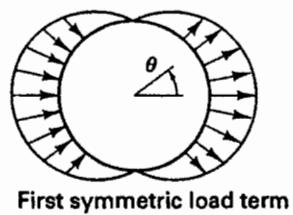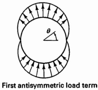EXAMPLE 4.20: Figure E4.20 shows an axisymmetric structure subjected to a nonaxisymmetric loading in the radial direction. Discuss the analysis of this structure using the three-node axisymmetric element in Example 4.17 when the loading is represented as a superposition of Fourier components. The stress distribution in the structure is three-dimensional and could be calculated using a three-dimensional finite element idealization. However, it is possible to take advantage of the axisymmetric geometry of the structure and, depending on the exact loading applied, reduce the computational effort very significantly. The key point in this analysis is that we expand the externally applied loads $R_{r}(\theta,y)$ in the Fourier series: $$ R _ {r} = \sum_ {p = 1} ^ {p _ {c}} R _ {p} ^ {c} \cos p \theta + \sum_ {p = 1} ^ {p _ {s}} R _ {p} ^ {s} \sin p \theta \tag {a} $$ 

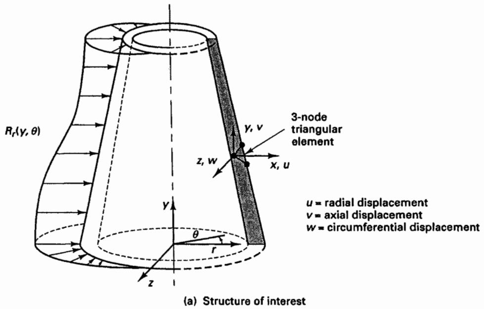
text_image

Rr(y, θ) y, v 3-node triangular element x, u z, w u = radial displacement v = axial displacement w = circumferential displacement θ r z (a) Structure of interest


text_image

First symmetric load term


text_image

First antisymmetric load term

(b) Representation of nonaxisymmetric loading Figure E4.20 Axisymmetric structure subjected to nonaxisymmetric loading where $p_{c}$ and $p_{s}$ are the total number of symmetric and antisymmetric load contributions about $\theta = 0$ , respectively. Figure E4.20(b) illustrates the first terms in the expansion of (a). The complete analysis can now be performed by superimposing the responses due to the symmetric and antisymmetric load contributions defined in (a). For example, considering the symmetric response, we use for an element $$ u (x, y, \theta) = \sum_ {p = 1} ^ {p _ {c}} \cos p \theta \mathbf {H} \hat {\mathbf {u}} ^ {p} $$ $$ v (x, y, \theta) = \sum_ {p = 1} ^ {p _ {c}} \cos p \theta \mathbf {H} \hat {\mathbf {v}} ^ {p} \tag {b} $$ $$ w (x, y, \theta) = \sum_ {p = 1} ^ {p _ {c}} \sin p \theta \mathbf {H} \hat {\mathbf {w}} ^ {p} $$ where for the triangular elements, referring to Example 4.17, $$ \mathbf {H} = \left[ \begin{array}{l l l} 1 & x & y \end{array} \right] \mathbf {A} _ {1} ^ {- 1} \tag {c} $$ and the $\hat{\mathbf{u}}^p$ , $\hat{\mathbf{v}}^p$ , and $\hat{\mathbf{w}}^p$ are the element unknown generalized nodal point displacements corresponding to mode $p$ . We should note that we superimpose in (b) the response measured in individual harmonic displacement distributions. Using (b), we can now establish the strain-displacement matrix of the element. Since we are dealing with a three-dimensional stress distribution, we use the expression for three-dimensional strain distributions in cylindrical coordinates: $$ \epsilon = \left[ \begin{array}{l} \frac {\partial u}{\partial r} \\ \frac {\partial v}{\partial y} \\ \frac {u}{r} + \frac {1}{r} \frac {\partial w}{\partial \theta} \\ \frac {\partial u}{\partial y} + \frac {\partial v}{\partial r} \\ \frac {\partial w}{\partial y} + \frac {1}{r} \frac {\partial v}{\partial \theta} \\ \frac {\partial w}{\partial r} + \frac {1}{r} \frac {\partial u}{\partial \theta} - \frac {w}{r} \end{array} \right] \tag {d} $$ where $\pmb{\epsilon}^{T} = [\pmb{\epsilon}_{rr}\quad \pmb{\epsilon}_{yy}\quad \pmb{\epsilon}_{\theta \theta}\quad \gamma_{ry}\quad \gamma_{y\theta}\quad \gamma_{\theta r}]$ (e) Substituting from (b) into (d) we obtain a strain-displacement matrix $B_{p}$ for each value of p, and the total strains can be thought of as the superposition of the strain distributions contained in each harmonic. The unknown nodal point displacements can now be evaluated using the usual procedures. The equilibrium equations corresponding to the generalized nodal point displacements $U_{i}^{p}$ , $V_{i}^{p}$ , $W_{i}^{p}$ , $i = 1, \ldots, N$ (N is equal to the total number of nodes) and $p = 1, \ldots, p_{c}$ are evaluated as given in (4.17) to (4.22), where we now have $$ \mathbf {U} ^ {T} = \left[ \begin{array}{l l l l} \mathbf {U} ^ {1 T} & \mathbf {U} ^ {2 T} & \dots & \mathbf {U} ^ {p _ {c} T} \end{array} \right] \tag {f} $$ and $$ \mathbf {U} ^ {p ^ {T}} = \left[ \begin{array}{l l l l l l l} U _ {1} ^ {p} & V _ {1} ^ {p} & W _ {1} ^ {p} & \vdots & U _ {2} ^ {p} & \dots & W _ {N} ^ {p} \end{array} \right] \tag {g} $$ In the calculations of K and $R_{s}$ we note that because of the orthogonality properties $$ \int_ {0} ^ {2 \pi} \sin n \theta \sin m \theta d \theta = 0 \quad n \neq m \tag {h} $$ $$ \int_ {0} ^ {2 \pi} \cos n \theta \cos m \theta d \theta = 0 \quad n \neq m $$ the stiffness matrices corresponding to the different harmonics are decoupled from each other. Hence, we have the following equilibrium equations for the structure: $$ \mathbf {K} ^ {p} \mathbf {U} ^ {p} = \mathbf {R} _ {S} ^ {p} \quad p = 1, \dots , p _ {c} \tag {i} $$ where $\mathbf{K}^p$ and $\mathbf{R}_S^p$ are the stiffness matrix and load vector corresponding to the $p$ th harmonic. Solution of the equations in (i) gives the generalized nodal point displacements of each element, and (b) then yields all element internal displacements. In the above displacement solution we considered only the symmetric load contributions. But an analogous analysis can be performed for the antisymmetric load harmonics of (a) by simply replacing in (b) to (i) all sine and cosine terms by cosine and sine terms, respectively. The complete structural response is then obtained by superimposing the displacements corresponding to all harmonics. Although we have considered only surface loading in the discussion, the analysis can be extended using the same approach to include body force loading and initial stresses. Finally, we note that the computational effort required in the analysis is directly proportional to the number of load harmonics used. Hence, the solution procedure is very efficient if the loading can be represented using only a few harmonics (e.g., wind loading) but may be inefficient when many harmonics must be used to represent the loading (e.g., a concentrated force). # 4.2.4 Lumping of Structure Properties and Loads A physical interpretation of the finite element procedure of analysis as presented in the previous sections is that the structure properties—stiffness and mass—and the loads, internal and external, are lumped to the discrete nodes of the element assemblage using the virtual work principle. 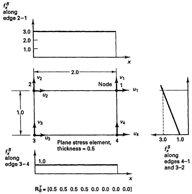Because the same interpolation functions are employed in the  Figure 4.6 Body force distribution and corresponding lumped body force vector $R_{B}$ of a rectangular element calculation of the load vectors and the mass matrix as in the evaluation of the stiffness matrix, we say that “consistent” load vectors and a consistent mass matrix are evaluated. In this case, provided certain conditions are fulfilled (see Section 4.3.3), the finite element solution is a Ritz analysis. It may now be recognized that instead of performing the integrations leading to the consistent load vector, we may evaluate an approximate load vector by simply adding to the actually applied concentrated nodal forces $R_{c}$ additional forces that are in some sense equivalent to the distributed loads on the elements. A somewhat obvious way of constructing approximate load vectors is to calculate the total body and surface forces corresponding to an element and to assign equal parts to the appropriate element nodal degrees of freedom. Consider as an example the rectangular plane stress element in Fig. 4.6 with the variation of the body force shown. The total body force is equal to 2.0, and hence we obtain the lumped body force vector given in the figure. In considering the derivation of an element mass matrix, we recall that the inertia forces have been considered part of the body forces. Hence we may also establish an approximate mass matrix by lumping equal parts of the total element mass to the nodal points. Realizing that each nodal mass essentially corresponds to the mass of an element contributing volume around the node, we note that using this procedure of lumping mass, we assume in essence that the accelerations of the contributing volume to a node are constant and equal to the nodal values. An important advantage of using a lumped mass matrix is that the matrix is diagonal, and, as will be seen later, the numerical operations for the solution of the dynamic equations of equilibrium are in some cases reduced very significantly. EXAMPLE 4.21: Evaluate the lumped body force vector and the lumped mass matrix of the element assemblage in Fig. E4.5. The lumped mass matrix is $$ \mathbf {M} = \rho \int_ {0} ^ {1 0 0} (1) \left[ \begin{array}{l l l} \frac {1}{2} & 0 & 0 \\ 0 & \frac {1}{2} & 0 \\ 0 & 0 & 0 \end{array} \right] d x + \rho \int_ {0} ^ {8 0} \left(1 + \frac {x}{4 0}\right) ^ {2} \left[ \begin{array}{l l l} 0 & 0 & 0 \\ 0 & \frac {1}{2} & 0 \\ 0 & 0 & \frac {1}{2} \end{array} \right] d x $$ $$ \mathbf {M} = \frac {\rho}{3} \left[ \begin{array}{c c c} 1 5 0 & 0 & 0 \\ 0 & 6 7 0 & 0 \\ 0 & 0 & 5 2 0 \end{array} \right] $$ Similarly, the lumped body force vector is $$ \begin{array}{l} \mathbf {R} _ {B} = \left(\int_ {0} ^ {1 0 0} (1) \left[ \begin{array}{l} \frac {1}{2} \\ \frac {1}{2} \\ 0 \end{array} \right] (1) d x + \int_ {0} ^ {8 0} \left(1 + \frac {x}{4 0}\right) ^ {2} \left[ \begin{array}{l} 0 \\ \frac {1}{2} \\ \frac {1}{2} \end{array} \right] \left(\frac {1}{1 0}\right) d x\right) f _ {2} (t) \\ = \frac {1}{3} \left[ \begin{array}{l} 1 5 0 \\ 2 0 2 \\ 5 2 \end{array} \right] f _ {2} (t) \\ \end{array} $$ It may be noted that, as required, the sums of the elements in M and $R_{B}$ in both this example and in Example 4.5 are the same.