where $^{0}s(r)$ is the arc length at time 0 of the material point $^{0}x_{1}(r)$ , $^{0}x_{2}(r)$ , $^{0}x_{3}(r)$ given by $$ { } ^ { 0 } s ( r ) = \sum _ { k = 1 } ^ { N } h _ { k } { } ^ { 0 } s _ { k } \tag {6.111} $$ The increment in the strain component $\tilde{t}_{0}\tilde{\epsilon}_{11}$ is denoted as $_{0}\tilde{\epsilon}_{11}$ , where $_{0}\tilde{\epsilon}_{11} = _{0}\tilde{e}_{11} + _{0}\tilde{\eta}_{11}$ and $$ _ 0 \tilde {e} _ {1 1} = \frac {d ^ {0} x _ {i}}{d ^ {0} s} \frac {d u _ {i}}{d ^ {0} s} + \frac {d ^ {\prime} u _ {i}}{d ^ {0} s} \frac {d u _ {i}}{d ^ {0} s} \tag {6.112} $$ $$ _ 0 \bar {\eta} _ {1 1} = \frac {1}{2} \frac {d u _ {i}}{d ^ {0} s} \frac {d u _ {i}}{d ^ {0} s} \tag {6.113} $$ For the strain-displacement matrices we define $$ { } ^ { 0 } \hat { \mathbf { X } } ^ { T } = \left[ { } ^ { 0 } x _ { 1 } ^ { 1 } \quad { } ^ { 0 } x _ { 2 } ^ { 1 } \quad { } ^ { 0 } x _ { 3 } ^ { 1 } \quad \cdots \quad { } ^ { 0 } x _ { 1 } ^ { N } \quad { } ^ { 0 } x _ { 2 } ^ { N } \quad { } ^ { 0 } x _ { 3 } ^ { N } \right] \tag {6.114} $$ $$ ^ {\prime} \hat {\mathbf {u}} ^ {T} = \left[ ^ {\prime} u _ {1} ^ {1} \quad^ {\prime} u _ {2} ^ {1} \quad^ {\prime} u _ {3} ^ {1} \quad \dots \quad^ {\prime} u _ {1} ^ {N} \quad^ {\prime} u _ {2} ^ {N} \quad^ {\prime} u _ {3} ^ {N} \right] $$ $$ \hat {\mathbf {u}} ^ {T} = \left[ u _ {1} ^ {1} \quad u _ {2} ^ {1} \quad u _ {3} ^ {1} \quad \dots \quad u _ {1} ^ {N} \quad u _ {2} ^ {N} \quad u _ {3} ^ {N} \right] \tag {6.115} $$ $$ \mathbf {H} = \left[ \begin{array}{c c c c c} h _ {1} \mathbf {I} _ {3} & \vdots & \dots & \vdots & h _ {N} \mathbf {I} _ {3} \end{array} \right]; \quad \mathbf {I} _ {3} = \left[ \begin{array}{c c c} 1 & 0 & 0 \\ 0 & 1 & 0 \\ 0 & 0 & 1 \end{array} \right] \tag {6.116} $$ and hence, using (6.112) and (6.113), $$ { } _ { 0 } ^ { t } \mathbf { B } _ { L } = ( ^ { 0 } J ^ { - 1 } ) ^ { 2 } ( ^ { 0 } \hat { \mathbf { x } } ^ { T } \mathbf { H } _ { , r } ^ { T } \mathbf { H } _ { , r } + { } ^ { t } \hat { \mathbf { u } } ^ { T } \mathbf { H } _ { , r } ^ { T } \mathbf { H } _ { , r } ) \tag {6.117} $$ and $t_0\mathbf{B}_{NL} = {}^0 J^{-1}\mathbf{H}_r$ (6.118) where $^{0}J^{-1}=dr/d^{0}s$ . We note that since $_{0}B_{NL}$ is independent of the orientation of the element, the matrix $_{0}K_{NL}$ is so as well. The only nonzero stress component is $\dot{t}_{0}\tilde{S}_{11}$ , which we assume to be given as a function of the Green-Lagrange strain $\dot{t}\tilde{\epsilon}_{11}$ at time t (see Section 6.6). The tangent stress-strain relationship is therefore $$ _ 0 \tilde {C} _ {1 1 1 1} = \frac {\partial_ {0} ^ {\prime} \tilde {S} _ {1 1}}{\partial_ {0} ^ {\prime} \tilde {\epsilon} _ {1 1}} \tag {6.119} $$ Using (6.114) to (6.119), the truss element matrices can be directly calculated as given in Table 6.4. Referring to Tables 6.2 to 6.4, the above relations can also be directly employed to develop the UL formulation, and of course the materially-nonlinear-only formulation. Consider the following examples. 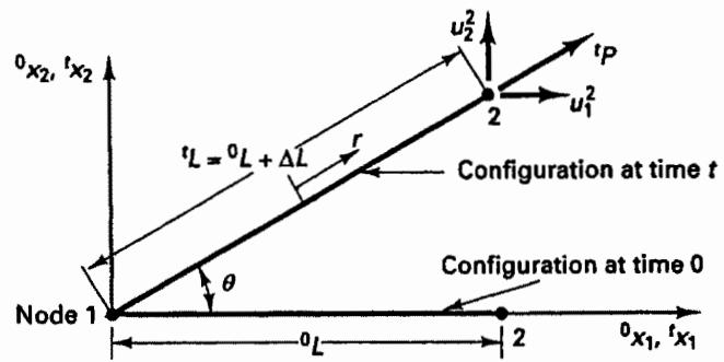EXAMPLE 6.16: For the two-node truss element shown in Fig. E6.16 develop the tangent stiffness matrix and force vector corresponding to the configuration at time t. Consider large displacement and large strain conditions. We note that the element is straight and is at time 0 aligned with the $^{0}x_{1}$ axis. Hence, we need not use the curl on the stress and strain components, and the equations of the formulation are somewhat simpler than (6.110) to (6.119). In the following we use two formulation approaches to emphasize some important points. 

text_image

0x2, tX2 tL = 0L + ΔL r Configuration at time t 0L θ Node 1 2 u2^2 u1^2 tP Configuration at time 0 0x1, tX1

(a) Two-node element 

text_image

Corresponds to elements in matrix t₀KNL (Δ is very small) (tP/tL Δ) tP Δ tL (tP/tL Δ) tP

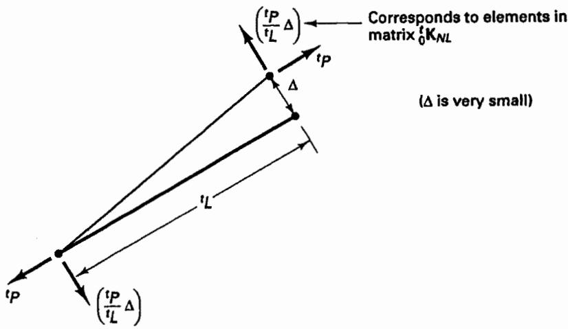
(b) Moment equilibrium of element Figure E6.16 Formulation of two-node truss element First Approach: Evaluation of Element Matrices Using Table 6.4: Using the TL formulation we need to express the strains $_{0}e_{11}$ and $_{0}\eta_{11}$ given in Table 6.2 [and (6.112) and (6.113)] in terms of the element displacement functions. Since the truss element undergoes displacements only in the $^{0}x_{1}$ , $^{0}x_{2}$ plane, we have $$ _ 0 e _ {1 1} = \frac {\partial u _ {1}}{\partial^ {0} x _ {1}} + \frac {\partial^ {t} u _ {1}}{\partial^ {0} x _ {1}} \frac {\partial u _ {1}}{\partial^ {0} x _ {1}} + \frac {\partial^ {t} u _ {2}}{\partial^ {0} x _ {1}} \frac {\partial u _ {2}}{\partial^ {0} x _ {1}} $$ $$ _ 0 \eta_ {1 1} = \frac {1}{2} \left[ \left(\frac {\partial u _ {1}}{\partial^ {0} x _ {1}}\right) ^ {2} + \left(\frac {\partial u _ {2}}{\partial^ {0} x _ {1}}\right) ^ {2} \right] $$ But by geometry, or using $u_{i} = \Sigma_{k=1}^{2} h_{k} u_{i}^{k}$ with $u_{1}^{1} = 0$ , $u_{2}^{1} = 0$ , $u_{1}^{2} = (^{0}L + \Delta L) \cos \theta - ^{0}L$ , $u_{2}^{2} = (^{0}L + \Delta L) \sin \theta$ , $^{0}J = ^{0}L / 2$ and the interpolation functions given in Fig. 5.3, we obtain $$ \frac {\partial^ {t} u _ {1}}{\partial^ {0} x _ {1}} = \frac {\left(^ {0} L + \Delta L\right) \cos \theta}{^ {0} L} - 1; \quad \frac {\partial^ {t} u _ {2}}{\partial^ {0} x _ {1}} = \frac {\left(^ {0} L + \Delta L\right) \sin \theta}{^ {0} L} $$ We therefore have $$ _ 0 e _ {1 1} = \frac {1}{^ 0 L} \left\{\left[ - 1 \quad 0 \quad 1 \quad 0 \right] + \left(\frac {{} ^ {0} L + \Delta L}{^ 0 L} \cos \theta - 1\right) \left[ - 1 \quad 0 \quad 1 \quad 0 \right] \right. $$ $$ \left. + \left(\frac {{} ^ {0} L + \Delta L}{^ {0} L} \sin \theta\right) [ 0 - 1 0 1 ] \right\} \left[ \begin{array}{l} u _ {1} ^ {1} \\ u _ {2} ^ {1} \\ u _ {1} ^ {2} \\ u _ {2} ^ {2} \end{array} \right] $$ $$ = \frac {{} ^ {0} L + \Delta L}{\left(^ {0} L\right) ^ {2}} \left[ - \cos \theta - \sin \theta \cos \theta \sin \theta \right] \left[ \begin{array}{l} u _ {1} ^ {1} \\ u _ {2} ^ {1} \\ u _ {1} ^ {2} \\ u _ {2} ^ {2} \end{array} \right] $$ and hence, $$ { } _ { 0 } ^ { t } \mathbf { B } _ { L } = \frac { { } ^ { 0 } L + \Delta L } { ( { } ^ { 0 } L ) ^ { 2 } } [ - \cos \theta - \sin \theta \cos \theta \sin \theta ] $$ Of course, the same result for $\delta \mathbf{B}_L$ is obtained using (6.117). The nonlinear strain displacement matrix is [from (6.118)] $$ { } _ { 0 } ^ { t } \mathbf { B } _ { N L } = \frac { 1 } { ^ { 0 } L } \left[ \begin{array} { c c c c } - 1 & 0 & 1 & 0 \\ 0 & - 1 & 0 & 1 \end{array} \right] $$ In the total Lagrangian formulation we assume that $\delta S_{11}$ is given in terms of $\delta \epsilon_{11}$ , and we have $$ _ 0 C _ {1 1 1 1} = \frac {\partial_ {0} ^ {t} S _ {1 1}}{\partial_ {0} ^ {t} \epsilon_ {1 1}} $$ If we use $_0^t S_{11} = E_0^t \epsilon_{11}$ , we have of course $_0^t C_{1111} = E$ . The tangent stiffness matrix and force vector are therefore (see Table 6.4) $$ { } _ { 0 } ^ { t } \mathbf { K } = { } _ { 0 } C _ { 1 1 1 1 } \frac { ( ^ { 0 } L + \Delta L ) ^ { 2 } } { ( ^ { 0 } L ) ^ { 3 } } { } ^ { 0 } A \left[ \begin{array} { c c c c } \cos ^ { 2 } \theta & \cos \theta \sin \theta & - \cos ^ { 2 } \theta & - \cos \theta \sin \theta \\ & \sin ^ { 2 } \theta & - \sin \theta \cos \theta & - \sin ^ { 2 } \theta \\ & & \cos ^ { 2 } \theta & \sin \theta \cos \theta \\ \text {Symmetric} & & & \sin ^ { 2 } \theta \end{array} \right] $$ $$ + \frac {^ t P}{^ 0 L + \Delta L} \left[ \begin{array}{c c c c} 1 & 0 & - 1 & 0 \\ 0 & 1 & 0 & - 1 \\ - 1 & 0 & 1 & 0 \\ 0 & - 1 & 0 & 1 \end{array} \right] \tag {a} $$ $$ { } _ { 0 } ^ { t } \mathbf { F } = { } ^ { \prime } P \left[ \begin{array} { c } - \cos \theta \\ - \sin \theta \\ \cos \theta \\ \sin \theta \end{array} \right] $$ where $^tP$ is the current force carried in the truss element. Here we have used, with the Cauchy stress equal to $^tP / ^tA$ , $$ { } _ { 0 } ^ { t } S _ { 1 1 } = \frac { { } ^ { 0 } \rho } { { } ^ { t } \rho } \left( \frac { { } ^ { 0 } L } { { } ^ { 0 } L + \Delta L } \right) ^ { 2 } \frac { { } ^ { t } P } { { } ^ { t } A } ; \quad { } _ { 0 } ^ { t } \epsilon _ { 1 1 } = \frac { \Delta L } { { } ^ { 0 } L } + \frac { 1 } { 2 } \left( \frac { \Delta L } { { } ^ { 0 } L } \right) ^ { 2 } $$ $$ { } ^ { 0 } \rho { } ^ { 0 } L { } ^ { 0 } A = { } ^ { \prime } \rho ( { } ^ { 0 } L + \Delta L ) { } ^ { \prime } A ; \quad { } _ { 0 } ^ { \prime } S _ { 1 1 } = \frac { { } ^ { 0 } L } { { } ^ { 0 } L + \Delta L } \frac { { } ^ { \prime } P } { { } ^ { 0 } A } \tag {b} $$ $$ ^ {\prime} P = _ {0} ^ {\prime} S _ {1 1} ^ {0} A \frac {{} ^ {0} L + \Delta L}{^ {0} L} $$ The first term in (a) represents the linear strain stiffness matrix, and the second term is the nonlinear strain stiffness matrix, which, as noted earlier, is independent of the angle $\theta$ . Second Approach: Taking the Derivative of the Force Vector $\delta \mathbf{F}$ : The tangent stiffness matrix of any element can be obtained by direct differentiation of the force vector $\delta \mathbf{F}$ (see Section 6.3.1); that is, $$ { } _ { 0 } ^ { t } \mathbf { K } = \frac { \partial _ { 0 } ^ { t } \mathbf { F } } { \partial ^ { t } \hat { \mathbf { u } } } \tag {c} $$ where $\hat{u}$ is the vector of nodal point displacements corresponding to time t. Here we have for the general truss element formulation in (6.106) to (6.119), $\hat{0}F = \int_{0_{V}} \hat{0}B_{L}^{T} \hat{0} \tilde{S}_{11} d^{0}V$ , so that $$ \frac {\partial_ {0} ^ {t} \mathbf {F}}{\partial^ {t} \hat {\mathbf {u}}} = \int_ {0 _ {V}} \delta \mathbf {B} \tilde {L} \frac {\partial_ {0} ^ {t} \tilde {S} _ {1 1}}{\partial_ {0} ^ {t} \tilde {\epsilon} _ {1 1}} \frac {\partial_ {0} ^ {t} \tilde {\epsilon} _ {1 1}}{\partial^ {t} \hat {\mathbf {u}}} d ^ {0} V + \int_ {0 _ {V}} \frac {\partial_ {0} ^ {t} \mathbf {B} \tilde {L}}{\partial^ {t} \hat {\mathbf {u}}} \delta \tilde {S} _ {1 1} d ^ {0} V \tag {d} $$ Using (6.117) and (6.118), we have $$ \frac {\partial_ {0} ^ {t} \mathbf {B} _ {L} ^ {T}}{\partial^ {t} \hat {\mathbf {u}}} = (^ {0} J ^ {- 1}) ^ {2} \mathbf {H} _ {, r} ^ {T} \mathbf {H} _ {, r} = _ {0} ^ {t} \mathbf {B} _ {N L} ^ {T} _ {0} ^ {t} \mathbf {B} _ {N L} $$ so that the second term in (d) gives the $\mathbf{0}\mathbf{K}_{NL}$ matrix. Also, using (6.110) and (6.117), we directly see that $$ \frac {\partial_ {0} ^ {\prime} \tilde {\epsilon} _ {1 1}}{\partial^ {\prime} \hat {\mathbf {u}}} = _ {0} ^ {\prime} \mathbf {B} _ {L} $$ and hence, the first term in (d) gives the $\delta \mathbf{K}_L$ matrix. However, to gain more insight, let us consider the derivation of ${}^{t}_{0}K$ in (c) specifically for the two-node truss element in Fig. E6.16 using the following details. For the two-node element, $\mathbf{f}$ is given by simple equilibrium $$ { } _ { 0 } ^ { \prime } \mathbf { F } = { } ^ { \prime } P \left[ \begin{array} { c } - \cos \theta \\ - \sin \theta \\ \cos \theta \\ \sin \theta \end{array} \right] $$ where $P$ is the current force (positive when a tensile force) carried by the element, and we have $$ ^ {\prime} \hat {\mathbf {u}} ^ {T} = \left[ ^ {\prime} u _ {1} ^ {1} \quad^ {\prime} u _ {2} ^ {1} \quad^ {\prime} u _ {1} ^ {2} \quad^ {\prime} u _ {2} ^ {2} \right] $$ Let us consider the third and fourth columns of the stiffness matrix (from which the first and second columns can be derived). We have $$ ^ \prime u _ {1} ^ {2} = (^ {0} L + \Delta L) \cos \theta - ^ {0} L $$ $$ ^ {\prime} u _ {2} ^ {2} = (^ {0} L + \Delta L) \sin \theta $$ and hence, $\left[ \begin{array}{c}\frac{\partial}{\partial(\Delta L)}\\ \frac{\partial}{\partial\theta} \end{array} \right] = \left[ \begin{array}{cc}\cos \theta & \sin \theta \\ -(^0 L + \Delta L)\sin \theta & (^0 L + \Delta L)\cos \theta \end{array} \right]\left[ \begin{array}{c}\frac{\partial}{\partial^t u_1^2}\\ \frac{\partial}{\partial^t u_2^2} \end{array} \right]$ from which $\left[ \begin{array}{c}\frac{\partial}{\partial^{\prime}u_{1}^{2}}\\ \frac{\partial}{\partial^{\prime}u_{2}^{2}} \end{array} \right] = \left[ \begin{array}{cc}\cos \theta & -\frac{\sin \theta}{^0L + \Delta L}\\ \sin \theta & \frac{\cos \theta}{^0L + \Delta L} \end{array} \right]\left[ \begin{array}{c}\frac{\partial}{\partial(\Delta L)}\\ \frac{\partial}{\partial\theta} \end{array} \right]$ Therefore, the third column of $\delta \mathbf{K}$ is given by $$ \begin{array}{l} \frac {\partial_ {0} ^ {t} \mathbf {F}}{\partial^ {\prime} u _ {1} ^ {2}} = \frac {\partial_ {0} ^ {t} \mathbf {F}}{\partial (\Delta L)} \frac {\partial (\Delta L)}{\partial^ {\prime} u _ {1} ^ {2}} + \frac {\partial_ {0} ^ {t} \mathbf {F}}{\partial \theta} \frac {\partial \theta}{\partial^ {\prime} u _ {1} ^ {2}} \\ = \frac {\partial^ {\prime} P}{\partial (\Delta L)} \left[ \begin{array}{c} - \cos \theta \\ - \sin \theta \\ \cos \theta \\ \sin \theta \end{array} \right] \cos \theta + ^ {\prime} P \left[ \begin{array}{c} \sin \theta \\ - \cos \theta \\ - \sin \theta \\ \cos \theta \end{array} \right] \left(\frac {- \sin \theta}{^ {0} L + \Delta L}\right) \tag {e} \\ = \frac {\partial \left(\frac {^ {\prime} P}{^ {0} L + \Delta L}\right)}{\partial (\Delta L)} (^ {0} L + \Delta L) \left[ \begin{array}{c} - \cos^ {2} \theta \\ - \sin \theta \cos \theta \\ \cos^ {2} \theta \\ \sin \theta \cos \theta \end{array} \right] + \frac {^ {\prime} P}{^ {0} L + \Delta L} \left[ \begin{array}{c} - 1 \\ 0 \\ 1 \\ 0 \end{array} \right] \\ \end{array} $$ Similarly, for the fourth column of $\delta \mathbf{K}$ , $$ \begin{array}{l} \frac {\partial_ {0} ^ {t} \mathbf {F}}{\partial^ {\prime} u _ {2} ^ {2}} = \frac {\partial_ {0} ^ {t} \mathbf {F}}{\partial (\Delta L)} \frac {\partial (\Delta L)}{\partial^ {\prime} u _ {2} ^ {2}} + \frac {\partial_ {0} ^ {t} \mathbf {F}}{\partial \theta} \frac {\partial \theta}{\partial^ {\prime} u _ {2} ^ {2}} \\ = \frac {\partial \left(\frac {^ \prime P}{^ 0 L + \Delta L}\right)}{\partial (\Delta L)} (^ {0} L + \Delta L) \left[ \begin{array}{c} - \cos \theta \sin \theta \\ - \sin^ {2} \theta \\ \sin \theta \cos \theta \\ \sin^ {2} \theta \end{array} \right] + \frac {^ \prime P}{^ 0 L + \Delta L} \left[ \begin{array}{c} 0 \\ - 1 \\ 0 \\ 1 \end{array} \right] \tag {f} \\ \end{array} $$ However, using (b), $$ \begin{array}{l} \frac {\partial \left(\frac {^ \prime P}{^ 0 L + \Delta L}\right)}{\partial (\Delta L)} (^ {0} L + \Delta L) = \frac {\partial^ {\prime} {} _ {0} S _ {1 1}}{\partial (\Delta L)} \frac {^ 0 L + \Delta L}{^ 0 L} ^ {0} A \\ = \frac {\partial_ {0} ^ {t} S _ {1 1}}{\partial_ {0} ^ {t} \epsilon_ {1 1}} \frac {\partial_ {0} ^ {t} \epsilon_ {1 1}}{\partial (\Delta L)} \frac {{} ^ {0} L + \Delta L}{^ {0} L} ^ {0} A = \frac {\partial_ {0} ^ {t} S _ {1 1}}{\partial_ {0} ^ {t} \epsilon_ {1 1}} \frac {\left(^ {0} L + \Delta L\right) ^ {2}}{^ {0} L ^ {3}} ^ {0} A \\ = _ {0} C _ {1 1 1 1} \frac {\left(^ {0} L + \Delta L\right) ^ {2}}{^ {0} L ^ {3}} ^ {0} A \\ \end{array} $$ $^{7}$ Note that if the material stress-strain relationship is such that $^{1}P$ is constant with changes in $\Delta L$ , only the second term in the second line of this equation is nonzero. Hence, the results in (e) and (f) are those already given in (a). We note that the entries in the nonlinear strain stiffness matrix can also be directly obtained from equilibrium considerations as shown in Fig. E6.16(b). Also, the updated Lagrangian formulation could be obtained from the result in (a) by using the relation (see Example 6.23) $$ { } _ { 0 } C _ { 1 1 1 1 } = \frac { { } ^ { 0 } \rho } { { } ^ { t } \rho } \left( \frac { { } ^ { 0 } L } { { } ^ { 0 } L + \Delta L } \right) ^ { 4 } , C _ { 1 1 1 1 } $$ so that in (a) $_{0}C_{1111}\frac{(^{0}L + \Delta L)^{2}}{(^{0}L)^{3}}{}^{0}A = {}_{t}C_{1111}\frac{{}^{t}A}{^0L + \Delta L}$ (g) If we also note that for infinitesimally small displacements the linear strain stiffness matrix reduces to the well-known truss element matrix (see Example 4.1), we recognize that with the result of (g) substituted in (a), the updated Lagrangian stiffness matrix is in fact what we would expect it to be from physical considerations. EXAMPLE 6.17: Establish the equilibrium equations used in the nonlinear analysis of the simple arch structure considered in Example 6.3 when the modified Newton-Raphson iteration is used for solution. In the modified Newton-Raphson iteration, we use (6.11) and (6.12) but evaluate new tangent stiffness matrices only at the beginning of each step. As in Example 6.3, we idealize the structure using one truss element [see Fig. E6.3(b)]. Since the displacements at node 1 are zero, we need to consider only the displacements at node 2. Using the derivations given in Example 6.16, with $\theta = {}^t\beta$ we have $$ { } _ { 0 } ^ { t } \mathbf { K } _ { L } = \frac { E A } { L } \left[ \begin{array} { c c } ( \cos ^ { t } \beta ) ^ { 2 } & \sin ^ { t } \beta \cos ^ { t } \beta \\ \sin ^ { t } \beta \cos ^ { t } \beta & ( \sin ^ { t } \beta ) ^ { 2 } \end{array} \right] $$ $$ { } _ { 0 } ^ { t } \mathbf { K } _ { N L } = \frac { { } ^ { t } P } { L } \left[ \begin{array} { c c } 1 & 0 \\ 0 & 1 \end{array} \right] $$ $$ { } _ { 0 } ^ { \prime } \mathbf { F } = { } ^ { \prime } P \left[ \begin{array} { c } \cos { { } ^ { \prime } \beta } \\ \sin { { } ^ { \prime } \beta } \end{array} \right] $$ where we assumed in the stiffness expressions that L and EA/L are constant throughout the response. The matrices correspond to the global displacements $u_1^2$ and $u_2^2$ at node 2. However, $u_1^2$ is zero, hence the governing equilibrium equation is $$ \left[ \frac {E A}{L} (\sin^ {\prime} \beta) ^ {2} + \frac {^ {t} P}{L} \right] \Delta u _ {2} ^ {2 (i)} = - \frac {^ {t + \Delta t} R}{2} - ^ {t + \Delta t} P ^ {(i - 1)} \sin (^ {t + \Delta t} \beta^ {(i - 1)}) $$ where $t^{+\Delta t}R/2$ is positive as shown in Fig. E6.3(b) and $t^{+\Delta t}P^{(i-1)}$ is the force in the bar (tensile force being positive) corresponding to the displacements at time $t + \Delta t$ and end of iteration $(i - 1)$ . 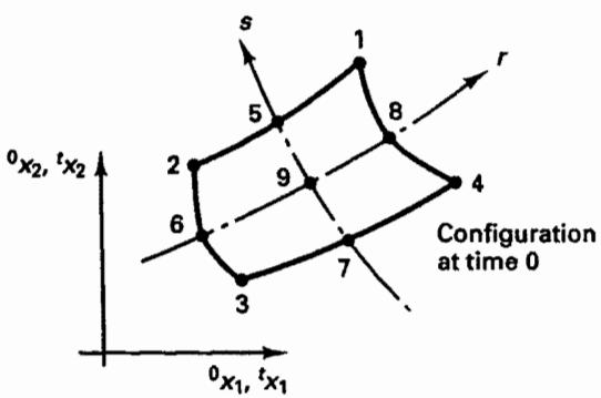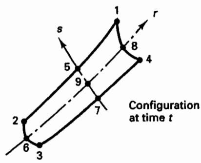# 6.3.4 Two-Dimensional Axisymmetric, Plane Strain, and Plane Stress Elements For the derivation of the required matrices and vectors, we consider a typical two-dimensional element in its configuration at time 0 and at time t, as illustrated for a nine-node element in Fig. 6.4. The global coordinates of the nodal points of the element are 

text_image

s 1 5 8 r 2 9 Configuration at time 0 6 3 7 4 0x2, tx2 0x1, tx1


text_image

s 1 r 8 5 9 4 2 7 Configuration at time t 6 3

Figure 6.4 Two-dimensional element shown in the global $x_{1}, x_{2}$ plane at time $0, ^0 x_1^k, ^0 x_2^k$ , and at time $t, ^t x_1^k, ^t x_2^k$ , where $k = 1, 2, \ldots, N$ , and $N$ denotes the total number of element nodes. Using the interpolation concepts discussed in Section 5.3, we have at time 0, $$ { } ^ { 0 } x _ { 1 } = \sum _ { k = 1 } ^ { N } h _ { k } { } ^ { 0 } x _ { 1 } ^ { k } ; \quad { } ^ { 0 } x _ { 2 } = \sum _ { k = 1 } ^ { N } h _ { k } { } ^ { 0 } x _ { 2 } ^ { k } \tag {6.120} $$ and at time $t$ $^t x_1 = \sum_{k=1}^{N} h_k^t x_1^k; \quad ^t x_2 = \sum_{k=1}^{N} h_k^t x_2^k$ (6.121) where the $h_k$ are the interpolation functions presented in Fig. 5.4. Since we use the isoparametric finite element discretization, the element displacements are interpolated in the same way as the geometry; i.e., $$ { } ^ { \prime } u _ { 1 } = \sum _ { k = 1 } ^ { N } h _ { k } { } ^ { \prime } u _ { 1 } ^ { k } ; \quad { } ^ { \prime } u _ { 2 } = \sum _ { k = 1 } ^ { N } h _ { k } { } ^ { \prime } u _ { 2 } ^ { k } \tag {6.122} $$ $$ u _ {1} = \sum_ {k = 1} ^ {N} h _ {k} u _ {1} ^ {k}; \quad u _ {2} = \sum_ {k = 1} ^ {N} h _ {k} u _ {2} ^ {k} \tag {6.123} $$ The evaluation of strains requires the following derivatives: $$ \frac {\partial^ {t} u _ {i}}{\partial^ {0} x _ {j}} = \sum_ {k = 1} ^ {N} \left(\frac {\partial h _ {k}}{\partial^ {0} x _ {j}}\right) ^ {t} u _ {i} ^ {k} \tag {6.124} $$ $$ \frac {\partial u _ {i}}{\partial^ {0} x _ {j}} = \sum_ {k = 1} ^ {N} \left(\frac {\partial h _ {k}}{\partial^ {0} x _ {j}}\right) u _ {i} ^ {k} \quad \begin{array}{l} i = 1, 2 \\ j = 1, 2 \end{array} \tag {6.125} $$ $$ \frac {\partial u _ {i}}{\partial^ {t} x _ {j}} = \sum_ {k = 1} ^ {N} \left(\frac {\partial h _ {k}}{\partial^ {t} x _ {j}}\right) u _ {i} ^ {k} \tag {6.126} $$ These derivatives are calculated in the same way as in linear analysis, i.e., using a Jacobian transformation. As an example, consider briefly the evaluation of the derivatives in (6.126). The other derivatives are obtained in an analogous manner. The chain rule relating $x_1, x_2$ , to $r, s$ derivatives is written as $$ \left[ \begin{array}{c} \frac {\partial}{\partial r} \\ \frac {\partial}{\partial s} \end{array} \right] = ^ {t} \mathbf {J} \left[ \begin{array}{c} \frac {\partial}{\partial^ {t} x _ {1}} \\ \frac {\partial}{\partial^ {t} x _ {2}} \end{array} \right] $$ in which $$ { } ^ { t } \mathbf { J } = \left[ \begin{array} { c c } \frac { \partial ^ { t } x _ { 1 } } { \partial r } & \frac { \partial ^ { t } x _ { 2 } } { \partial r } \\ \frac { \partial ^ { t } x _ { 1 } } { \partial s } & \frac { \partial ^ { t } x _ { 2 } } { \partial s } \end{array} \right] $$ Inverting the Jacobian operator J, we obtain $$ \left[ \begin{array}{c} \frac {\partial}{\partial^ {t} x _ {1}} \\ \frac {\partial}{\partial^ {t} x _ {2}} \end{array} \right] = \frac {1}{\det ^ {t} \mathbf {J}} \left[ \begin{array}{c c} \frac {\partial^ {t} x _ {2}}{\partial s} & - \frac {\partial^ {t} x _ {2}}{\partial r} \\ - \frac {\partial^ {t} x _ {1}}{\partial s} & \frac {\partial^ {t} x _ {1}}{\partial r} \end{array} \right] \left[ \begin{array}{c} \frac {\partial}{\partial r} \\ \frac {\partial}{\partial s} \end{array} \right] $$ where the Jacobian determinant is $$ \det ^ {\prime} \mathbf {J} = \frac {\partial^ {\prime} x _ {1}}{\partial r} \frac {\partial^ {\prime} x _ {2}}{\partial s} - \frac {\partial^ {\prime} x _ {1}}{\partial s} \frac {\partial^ {\prime} x _ {2}}{\partial r} $$ and the derivatives of the coordinates with respect to $r$ and $s$ are obtained as usual using (6.121); e.g., $$ \frac {\partial^ {\prime} x _ {1}}{\partial r} = \sum_ {k = 1} ^ {N} \frac {\partial h _ {k}}{\partial r} ^ {\prime} x _ {1} ^ {k} $$ With all required derivatives defined, it is now possible to establish the strain-displacement transformation matrices for the elements. Table 6.5 gives the required matrices for the UL and TL formulations. In the numerical integration these matrices are evaluated at the Gauss integration points (see Section 5.5). As we pointed out earlier, the choice between the TL and UL formulations essentially depends on their relative numerical effectiveness. Table 6.5 shows that all matrices of the two formulations have corresponding patterns of zero elements, except that $\mathbf{\delta}_{0}\mathbf{B}_{L}$ is a full matrix whereas $\mathbf{\delta}_{L}\mathbf{B}_{L}$ is sparse. The strain-displacement transformation matrix $\mathbf{\delta}_{0}\mathbf{B}_{L}$ is full because of the initial displacement effect in the linear strain terms (see Tables 6.2 and 6.3). Therefore, the calculation of the matrix product $\mathbf{\delta}_{L}^{\mathbf{T}}\mathbf{C}\mathbf{\delta}_{L}\mathbf{B}_{L}$ in the UL formulation requires less time than the calculation of the matrix product $\mathbf{\delta}_{L}^{\mathbf{T}}\mathbf{C}\mathbf{\delta}_{L}\mathbf{B}_{L}$ in the TL formulation. The second numerical difference between the two formulations is that in the TL formulation all derivatives of interpolation functions are with respect to the initial coordinates, whereas in the UL formulation all derivatives are with respect to the coordinates at time t. Therefore, in the TL formulation the derivatives could be calculated only once in the first load step and stored on back-up storage for use in all subsequent load steps. However, in practice, such storage can be expensive and in a computer implementation the derivatives of the interpolation functions are in general best recalculated in each time step. TABLE 6.5 Matrices used in the two-dimensional element formulation # A. Total Lagrangian formulation # 1. Incremental strains $$ \begin{array}{l} _ 0 \epsilon_ {1 1} = _ {0} u _ {1, 1} + _ {0} ^ {t} u _ {1, 1 0} u _ {1, 1} + _ {0} ^ {t} u _ {2, 1 0} u _ {2, 1} + \frac {1}{2} ((_ {0} u _ {1, 1}) ^ {2} + (_ {0} u _ {2, 1}) ^ {2}) \\ _ 0 \epsilon_ {2 2} = _ {0} u _ {2, 2} + _ {0} u _ {1, 2 0} u _ {1, 2} + _ {0} u _ {2, 2 0} u _ {2, 2} + \frac {1}{2} ((_ {0} u _ {1, 2}) ^ {2} + (_ {0} u _ {2, 2}) ^ {2}) \\ _ 0 \epsilon_ {1 2} = \frac {1}{2} (_ {0} u _ {1, 2} + _ {0} u _ {2, 1}) + \frac {1}{2} (_ {0} u _ {1, 1 0} u _ {1, 2} + _ {0} u _ {2, 1 0} u _ {2, 2} + _ {0} u _ {1, 2 0} u _ {1, 1} + _ {0} u _ {2, 2 0} u _ {2, 1}) + \frac {1}{2} (_ {0} u _ {1, 1 0} u _ {1, 2} + _ {0} u _ {2, 1 0} u _ {2, 2}) \\ _ 0 \epsilon_ {3 3} = \frac {u _ {1}}{^ 0 x _ {1}} + \frac {^ t u _ {1} u _ {1}}{\left(^ {0} x _ {1}\right) ^ {2}} + \frac {1}{2} \left(\frac {u _ {1}}{^ 0 x _ {1}}\right) ^ {2} \quad \text { for axisymmetric analysis } \\ \end{array} $$ $$ \text { where } _ {0} u _ {i, j} = \frac {\partial u _ {i}}{\partial^ {0} x _ {j}}; \quad \quad \quad \quad \quad \quad \quad \quad \quad \quad \quad \quad \quad \quad \quad \quad \quad \quad \quad \quad \quad \quad \quad \quad \quad \quad \quad \quad \quad \quad \quad \quad \quad \quad \quad \quad \quad \quad \quad \quad \quad \quad \quad \quad \quad \quad \quad \quad \quad \quad \text { or } \quad \quad \quad \quad \quad \quad \quad \quad \quad \quad \quad \quad \quad \quad \quad \quad \quad \quad \quad \quad \quad \quad \quad \quad \quad \quad \quad \quad \quad \quad \quad \quad \quad \quad \quad \quad \quad \quad \quad \quad \quad \quad \quad \quad \quad \quad \quad \quad \quad \tag {1.1} $$ # 2. Linear strain-displacement transformation matrix $$ \text { Using } _ {0} \mathbf {e} = \delta \mathbf {B} _ {L} \hat {\mathbf {u}} $$ $$ \text { where } _ {0} \mathbf {e} ^ {T} = \left[ \begin{array}{l l l l l} 0 e _ {1 1} & _ {0} e _ {2 2} & 2 _ {0} e _ {1 2} & _ {0} e _ {3 3} \end{array} \right]; \quad \hat {\mathbf {u}} ^ {T} = \left[ \begin{array}{l l l l l} u _ {1} ^ {1} & u _ {2} ^ {1} & u _ {1} ^ {2} & u _ {2} ^ {2} \dots u _ {1} ^ {N} & u _ {2} ^ {N} \end{array} \right] $$ $$ \text { and } \quad \mathbf {0} \mathbf {B} _ {L} = \mathbf {0} \mathbf {B} _ {L 0} + \mathbf {0} \mathbf {B} _ {L 1} $$ $$ \mathbf {0} \mathbf {B} _ {L 0} = \left[ \begin{array}{c c c c c c c c c} _ {0} h _ {1, 1} & 0 & _ {0} h _ {2, 1} & 0 & _ {0} h _ {3, 1} & 0 & \dots & _ {0} h _ {N, 1} & 0 \\ 0 & _ {0} h _ {1, 2} & 0 & _ {0} h _ {2, 2} & 0 & _ {0} h _ {3, 2} & \dots & 0 & _ {0} h _ {N, 2} \\ _ {0} h _ {1, 2} & _ {0} h _ {1, 1} & _ {0} h _ {2, 2} & _ {0} h _ {2, 1} & _ {0} h _ {3, 2} & _ {0} h _ {3, 1} & \dots & _ {0} h _ {N, 2} & _ {0} h _ {N, 1} \\ \frac {h _ {1}}{_ {0} \overline {{x}} _ {1}} & 0 & \frac {h _ {2}}{_ {0} \overline {{x}} _ {1}} & 0 & \frac {h _ {3}}{_ {0} \overline {{x}} _ {1}} & 0 & \dots & \frac {h _ {N}}{_ {0} \overline {{x}} _ {1}} & 0 \end{array} \right] $$ $$ \text { where } _ {0} h _ {k, j} = \frac {\partial h _ {k}}{\partial^ {0} x _ {j}}; \quad u _ {j} ^ {k} = ^ {t + \Delta t} u _ {j} ^ {k} - ^ {t} u _ {j} ^ {k}; \quad {} ^ {0} x _ {1} ^ {-} = \sum_ {k = 1} ^ {N} h _ {k} ^ {0} x _ {1} ^ {k}; \quad N = \text { number of nodes } $$ and $$ _ 0 \mathbf {B} _ {L 1} = \left[ \begin{array}{c c c c} l _ {1 1 0} h _ {1, 1} & l _ {2 1 0} h _ {1, 1} & l _ {1 1 0} h _ {2, 1} & l _ {2 1 0} h _ {2, 1} \\ l _ {1 2 0} h _ {1, 2} & l _ {2 2 0} h _ {1, 2} & l _ {1 2 0} h _ {2, 2} & l _ {2 2 0} h _ {2, 2} \\ \left(l _ {1 1 0} h _ {1, 2} + l _ {1 2 0} h _ {1, 1}\right) & \left(l _ {2 1 0} h _ {1, 2} + l _ {2 2 0} h _ {1, 1}\right) & \left(l _ {1 1 0} h _ {2, 2} + l _ {1 2 0} h _ {2, 1}\right) & \left(l _ {2 1 0} h _ {2, 2} + l _ {2 2 0} h _ {2, 1}\right) \\ l _ {3 3} \frac {h _ {1}}{0 \overline {{x _ {1}}}} & 0 & l _ {3 3} \frac {h _ {2}}{0 \overline {{x _ {1}}}} & 0 \end{array} \right. $$ $$ \left. \begin{array}{c c c} \dots & l _ {1 1 0} h _ {N, 1} & l _ {2 1 0} h _ {N, 1} \\ \dots & l _ {1 2 0} h _ {N, 2} & l _ {2 2 0} h _ {N, 2} \\ \dots & \left(l _ {1 1 0} h _ {N, 2} + l _ {1 2 0} h _ {N, 1}\right) & \left(l _ {2 1 0} h _ {N, 2} + l _ {2 2 0} h _ {N, 1}\right) \\ \dots & l _ {3 3} \frac {h _ {N}}{0 x _ {1}} & 0 \end{array} \right] $$ $$ \text { where } l _ {1 1} = \sum_ {k = 1} ^ {N} _ {0} h _ {k, 1} ^ {\prime} u _ {1} ^ {k}; \quad l _ {2 2} = \sum_ {k = 1} ^ {N} _ {0} h _ {k, 2} ^ {\prime} u _ {2} ^ {k}; \quad l _ {2 1} = \sum_ {k = 1} ^ {N} _ {0} h _ {k, 1} ^ {\prime} u _ {2} ^ {k}; \quad l _ {1 2} = \sum_ {k = 1} ^ {N} _ {0} h _ {k, 2} ^ {\prime} u _ {1} ^ {k}; $$ $$ l _ {3 3} = \frac {\sum_ {k = 1} ^ {N} h _ {k} ^ {\prime} u _ {1} ^ {k}}{0 \overline {{x}} _ {1}} $$ # 3. Nonlinear strain-displacement transformation matrix $$ \mathbf {0} \mathbf {B} _ {N L} = \left[ \begin{array}{c c c c c c c c c} _ {0} h _ {1, 1} & 0 & _ {0} h _ {2, 1} & 0 & _ {0} h _ {3, 1} & 0 & \dots & _ {0} h _ {N, 1} & 0 \\ _ {0} h _ {1, 2} & 0 & _ {0} h _ {2, 2} & 0 & _ {0} h _ {3, 2} & 0 & \dots & _ {0} h _ {N, 2} & 0 \\ 0 & _ {0} h _ {1, 1} & 0 & _ {0} h _ {2, 1} & 0 & _ {0} h _ {3, 1} & \dots & 0 & _ {0} h _ {N, 1} \\ 0 & _ {0} h _ {1, 2} & 0 & _ {0} h _ {2, 2} & 0 & _ {0} h _ {3, 2} & \dots & 0 & _ {0} h _ {N, 2} \\ \frac {h _ {1}}{_ {0} \overline {{x}} _ {1}} & 0 & \frac {h _ {2}}{_ {0} \overline {{x}} _ {1}} & 0 & \frac {h _ {3}}{_ {0} \overline {{x}} _ {1}} & 0 & \dots & \frac {h _ {N}}{_ {0} \overline {{x}} _ {1}} & 0 \end{array} \right] $$ # TABLE 6.5 (cont.) 4. Second Piola-Kirchhoff stress matrix and vector $$ \mathbf {s} \mathbf {S} = \left[ \begin{array}{c c c c c} \mathbf {s} _ {0} S _ {1 1} & \mathbf {b} S _ {1 2} & 0 & 0 & 0 \\ \mathbf {s} _ {0} S _ {2 1} & \mathbf {b} S _ {2 2} & 0 & 0 & 0 \\ 0 & 0 & \mathbf {b} S _ {1 1} & \mathbf {b} S _ {1 2} & 0 \\ 0 & 0 & \mathbf {b} S _ {2 1} & \mathbf {b} S _ {2 2} & 0 \\ 0 & 0 & 0 & 0 & \mathbf {b} S _ {3 3} \end{array} \right]; \quad \mathbf {s} \hat {\mathbf {S}} = \left[ \begin{array}{c} \mathbf {b} S _ {1 1} \\ \mathbf {b} S _ {2 2} \\ \mathbf {b} S _ {1 2} \\ \mathbf {b} S _ {3 3} \end{array} \right] $$ B. Updated Lagrangian formulation 1. Incremental strains $$ \begin{array}{l} _ {t} \epsilon_ {1 1} = _ {t} u _ {1, 1} + \frac {1}{2} \left(\left(_ {t} u _ {1, 1}\right) ^ {2} + \left(_ {t} u _ {2, 1}\right) ^ {2}\right) \\ _ {t} \epsilon_ {2 2} = _ {t} u _ {2, 2} + \frac {1}{2} ((_ {t} u _ {1, 2}) ^ {2} + (_ {t} u _ {2, 2}) ^ {2}) \\ \epsilon_ {1 2} = \frac {1}{2} \left(u _ {1, 2} + u _ {2, 1}\right) + \frac {1}{2} \left(u _ {1, 1}, u _ {1, 2} + u _ {2, 1}, u _ {2, 2}\right) \\ _ {t} \epsilon_ {3 3} = \frac {u _ {1}}{^ t x _ {1}} + \frac {1}{2} \left(\frac {u _ {1}}{^ t x _ {1}}\right) ^ {2} \quad \text { for axisymmetric analysis } \\ \end{array} $$ $$ \text { where } _ {i} u _ {i, j} = \frac {\partial u _ {i}}{\partial^ {\prime} x _ {j}} $$ 2. Linear strain-displacement transformation matrix $$ \text { Using } _ {t} \mathbf {e} = ; \mathbf {B} _ {L} \hat {\mathbf {u}} $$ $$ \text { where } _ {r} \mathbf {e} ^ {T} = [ _ {r} e _ {1 1} \quad_ {r} e _ {2 2} \quad 2 _ {r} e _ {1 2} \quad_ {r} e _ {3 3} ]; \quad \hat {\mathbf {u}} ^ {T} = [ u | \quad u _ {2} ^ {1} \quad u _ {1} ^ {2} \quad u _ {2} ^ {2} \quad \dots \quad u _ {1} ^ {N} \quad u _ {2} ^ {N} ] $$ $$ { } ^ { t } \mathbf { B } _ { L } = \left[ \begin{array} { c c c c c c c c c } { } _ { t } h _ { 1 , 1 } & 0 & { } _ { t } h _ { 2 , 1 } & 0 & { } _ { t } h _ { 3 , 1 } & 0 & \cdots & { } _ { t } h _ { N , 1 } & 0 \\ 0 & { } _ { t } h _ { 1 , 2 } & 0 & { } _ { t } h _ { 2 , 2 } & 0 & { } _ { t } h _ { 3 , 2 } & \cdots & 0 & { } _ { t } h _ { N , 2 } \\ { } _ { t } h _ { 1 , 2 } & { } _ { t } h _ { 1 , 1 } & { } _ { t } h _ { 2 , 2 } & { } _ { t } h _ { 2 , 1 } & { } _ { t } h _ { 3 , 2 } & { } _ { t } h _ { 3 , 1 } & \cdots & { } _ { t } h _ { N , 2 } & { } _ { t } h _ { N , 1 } \\ \frac { h _ { 1 } } { { } _ { t } \overline { { x } } _ { 1 } } & 0 & \frac { h _ { 2 } } { { } _ { t } \overline { { x } } _ { 1 } } & 0 & \frac { h _ { 3 } } { { } _ { t } \overline { { x } } _ { 1 } } & 0 & \cdots & \frac { h _ { N } } { { } _ { t } \overline { { x } } _ { 1 } } & 0 \end{array} \right] $$ $$ \text { where } _ {t} h _ {k, j} = \frac {\partial h _ {k}}{\partial^ {t} x _ {j}}; \quad u _ {j} ^ {k} = ^ {t + \Delta t} u _ {j} ^ {k} - ^ {t} u _ {j} ^ {k}; \quad^ {t} \bar {x} _ {1} = \sum_ {k = 1} ^ {N} h _ {k} ^ {t} x _ {1} ^ {k}; \quad N = \text { number of nodes } $$ 3. Nonlinear strain-displacement transformation matrix $$ { } _ { i } ^ { \prime } \mathbf { B } _ { N L } = \left[ \begin{array} { c c c c c c c c c } { } _ { i } h _ { 1 , 1 } & 0 & { } _ { i } h _ { 2 , 1 } & 0 & { } _ { i } h _ { 3 , 1 } & 0 & \cdots & { } _ { i } h _ { N , 1 } & 0 \\ { } _ { i } h _ { 1 , 2 } & 0 & { } _ { i } h _ { 2 , 2 } & 0 & { } _ { i } h _ { 3 , 2 } & 0 & \cdots & { } _ { i } h _ { N , 2 } & 0 \\ 0 & { } _ { i } h _ { 1 , 1 } & 0 & { } _ { i } h _ { 2 , 1 } & 0 & { } _ { i } h _ { 3 , 1 } & \cdots & 0 & { } _ { i } h _ { N , 1 } \\ 0 & { } _ { i } h _ { 1 , 2 } & 0 & { } _ { i } h _ { 2 , 2 } & 0 & { } _ { i } h _ { 3 , 2 } & \cdots & 0 & { } _ { i } h _ { N , 2 } \\ \frac { h _ { 1 } } { i \overline { { x } } _ { 1 } } & 0 & \frac { h _ { 2 } } { i \overline { { x } } _ { 1 } } & 0 & \frac { h _ { 3 } } { i \overline { { x } } _ { 1 } } & 0 & \cdots & \frac { h _ { N } } { i \overline { { x } } _ { 1 } } & 0 \end{array} \right] $$ 4. Cauchy stress matrix and stress vector $$ ^ {\prime} \boldsymbol {\tau} = \left[ \begin{array}{c c c c c} ^ {\prime} \tau_ {1 1} & ^ {\prime} \tau_ {1 2} & 0 & 0 & 0 \\ ^ {\prime} \tau_ {2 1} & ^ {\prime} \tau_ {2 2} & 0 & 0 & 0 \\ 0 & 0 & ^ {\prime} \tau_ {1 1} & ^ {\prime} \tau_ {1 2} & 0 \\ 0 & 0 & ^ {\prime} \tau_ {2 1} & ^ {\prime} \tau_ {2 2} & 0 \\ 0 & 0 & 0 & 0 & ^ {\prime} \tau_ {3 3} \end{array} \right]; \quad^ {\prime} \hat {\boldsymbol {\tau}} = \left[ \begin{array}{c} ^ {\prime} \tau_ {1 1} \\ ^ {\prime} \tau_ {2 2} \\ ^ {\prime} \tau_ {1 2} \\ ^ {\prime} \tau_ {3 3} \end{array} \right] $$