| Problem | Variable θ | Constants $k_x, k_y, k_z$ | Input $q^B$ | Input $q^S$ |
| Heat transfer | Temperature | Thermal conductivity | Internal heat generation | Prescribed heat flow |
| Seepage | Total head | Permeability | Internal flow generation | Prescribed flow condition |
| Torsion | Stress function | $(Shear modulus)^{-1}$ | 2 × (Angle of twist) | — |
| Inviscid incompressible irrotational flow | Potential function | 1 | Source or sink | Prescribed velocity |
| Electric conduction | Voltage | Electric conductivity | Internal current source | Prescribed current |
| Electrostatic field analysis | Field potential | Permittivity | Charge density | Prescribed field |
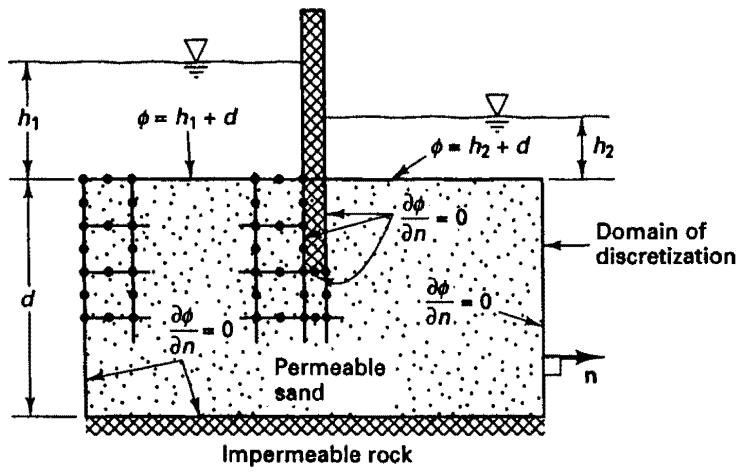
# 7.3.1 Seepage
The equations discussed in Section 7.2.1 are directly applicable in seepage analysis provided confined flow conditions are considered. In this case the boundary surfaces and boundary conditions are all known. To solve for unconfined flow conditions the position of the free surface must also be calculated, for which a special solution procedure needs to be employed (see C. S. Desai [A] and K. J. Bathe and M. R. Khoshgoftaar [B]).
The basic seepage law used in the analysis is Darcy's law, which gives the flow through the porous medium in terms of the gradient of the total potential $\phi$ (see, for example, A. Verruijt [A]),
$$
q _ {x} = - k _ {x} \frac {\partial \phi}{\partial x}; \quad q _ {y} = - k _ {y} \frac {\partial \phi}{\partial y}; \quad q _ {z} = - k _ {z} \frac {\partial \phi}{\partial z} \tag {7.37}
$$
Continuity of flow conditions then results in the equation
$$
\frac {\partial}{\partial x} \left(k _ {x} \frac {\partial \phi}{\partial x}\right) + \frac {\partial}{\partial y} \left(k _ {y} \frac {\partial \phi}{\partial y}\right) + \frac {\partial}{\partial z} \left(k _ {z} \frac {\partial \phi}{\partial z}\right) = - q ^ {B} \tag {7.38}
$$
where $k_{x}$ , $k_{y}$ , and $k_{z}$ are the permeabilities of the medium and $q^{B}$ is the flow generated per unit volume. The boundary conditions are those of a prescribed total potential $\phi$ on the surface $S_{\phi}$ ,
$$
\phi | _ {s _ {\phi}} = \phi^ {s} \tag {7.39}
$$
and of a prescribed flow condition along the surface $S_{q}$ ,
$$
k _ {n} \left. \frac {\partial \phi}{\partial n} \right| _ {s _ {q}} = q ^ {s} \tag {7.40}
$$
where n denotes the coordinate axis in the direction of the unit normal vector n (pointing outward) to the surface. In (7.38) to (7.40) we are employing the same notation as in (7.1) to (7.3), and on comparing these sets of equations we find a complete analogy between the