(IELEM, INODE) with the increment size factor, FACTO, being input for each increment. This permits unequal load increments to be taken. It should be noted that the applied loading at any instant is accumulative. Therefore, if FACTO is input for the first three increments as respectively 0·5, 0·3 and 0·1, the total loading applied to the structure during the third increment is 0·9 times the loading input in subroutine DATA. The above also holds for loading by incremental prescribed displacements. TOLER This item of data controls the tolerance permitted on the convergence process. Its use will be described in detail in Sections 3.9.2 and 3.9.3. Subroutine INCLOD is now presented and described: SUBROUTINE INCLOD INCL 1 C************************** INCL 2 C INCL 3 C *** INPUTS DATA FOR CURRENT INCREMENT AND UPDATES LOAD VECTOR INCL 4 C INCL 5 C************************** INCL 6 COMMON/UNIM1/NPOIN,NELEM,NBOUN,NLOAD,NPROP,NNODE,IINCS,IITER, INCL 7 KRESL,NCHEK,TOLER,NALGO,NSVAB,NDOFN,NINCS,NEVAB, INCL 8 NITER,NOUTP,FACTO,PVALU INCL 9 COMMON/UNIM2/PROPS(5,4),COORD(26),LNODS(25,2),IFPRE(52), INCL 10 FIXED(52),TLOAD(25,4),RLOAD(25,4),ELOAD(25,4), INCL 11 MATNO(25),STRES(25,2),PLAST(25),XDISP(52), INCL 12 TDISP(26,2),TREAC(26,2),ASTIF(52,52),ASLOD(52), INCL 13 REACT(52),FRESV(1352),PEFIX(52),ESTIF(4,4) INCL 14 READ (5,900) NITER,NOUTP,FACTO,TOLER INCL 15 900 FORMAT(2I5,2F15.5) INCL 16 WRITE(6,905) IINCS,NITER,NOUTP,FACTO,TOLER INCL 17 905 FORMAT(1H0,5X,'IINCS=',I5,3X,'NITER=',I5,3X,'NOUTP=',I5, INCL 18 3X,'FACTO=',E14.6,3X,'TOLER=',E14.6) INCL 19 DO 10 IELEM=1,NELEM INCL 20 DO 10 IEVAB=1,NEVAB INCL 21 ELOAD(IELEM,IEVAB)=ELOAD(IELEM,IEVAB)+RLOAD(IELEM,IEVAB)*FACTO INCL 22 TLOAD(IELEM,IEVAB)=TLOAD(IELEM,IEVAB)+RLOAD(IELEM,IEVAB)*FACTO INCL 23 10 CONTINUE INCL 24 RETURN INCL 25 END INCL 26 INCL 15–19 Read and write the input data required for each load increment as described previously in this section. INCL 20-24 Add the current increment of load into the out of balance load array ELOAD and the total applied load vector TLOAD. # 3.8 The master or controlling segment The final portion of the program which will be common to all four programs (subject to the minor differences indicated in Fig. 3.1) is the master segment which controls the calling, in order, of the other subroutines. This program segment also controls the iterative process and also the incrementing of the applied loads, where appropriate. The following channel numbers are employed by the programs: 5 (card reader), 6 (line printer), 1 (scratch file). The MASTER segment will now be presented in the form required in the next section for the solution of one-dimensional quasi-harmonic problems by direct iteration. For other applications it is only necessary to arrange for the calling of appropriate subroutines as indicated in Fig. 3.1. ```csv MASTER UNIDIM C***** C C *** PROGRAM FOR THE 1-D SOLUTION OF NONLINEAR PROBLEMS C C***** COMMON/UNIM1/NPOIN, NELEM, NBOUN, NLOAD, NPROP, NNODE, IINCS, IITER, KRESL, NCHEK, TOLER, NALGO, NSVAB, NDOFN, NINCS, NEVAB, NITER, NOUTP, FACTO, PVALU COMMON/UNIM2/PROPS(5,4), COORD(26), LNODS(25,2), IFPRE(52), FIXED(52), TLOAD(25,4), RLOAD(25,4), ELOAD(25,4), MATNO(25), STRES(25,2), PLAST(25), XDISP(52), TDISP(26,2), TREAC(26,2), ASTIF(52,52), ASLOD(52), REACT(52), FRESV(1352), PEFIX(52), ESTIF(4,4) CALL DATA CALL INITIAL DO 30 IINCS=1, NINCS CALL INCLOD DO 10 IITER=1, NITER CALL NONAL IF(KRESL.EQ.1) CALL STIFF1 CALL ASSEMB IF(KRESL.EQ.1) CALL GREDUC IF(KRESL.EQ.2) CALL RESOLV CALL BAKSUB CALL MONITR(RINTL) IF(NCHEK.EQ.0) GO TO 20 IF(IITER.EQ.1. AND.NOUTP.EQ.1) CALL RESULT IF(NOUTP.EQ.2) CALL RESULT 10 CONTINUE WRITE(6,900) 900 FORMAT(1H0,5X,'SOLUTION NOT CONVERGED') STOP 20 CALL RESULT 30 CONTINUE STOP END QUIT 1 QUIT 2 QUIT 3 QUIT 4 QUIT 5 QUIT 6 QUIT 7 QUIT 8 QUIT 9 QUIT 10 QUIT 11 QUIT 12 QUIT 13 QUIT 14 QUIT 15 QUIT 16 QUIT 17 QUIT 18 QUIT 19 QUIT 20 QUIT 21 QUIT 22 QUIT 23 QUIT 24 QUIT 25 QUIT 26 QUIT 27 QUIT 28 QUIT 29 QUIT 30 QUIT 31 QUIT 32 QUIT 33 QUIT 34 QUIT 35 QUIT 36 QUIT 37 ``` QUIT 15 Call the subroutine which reads the input data as described in Section 3.2. QUIT 16 Call the subroutine which initialises various arrays to zero. QUIT 17 Enter the DO LOOP over the number of load increments. QUIT 18 Call the subroutine which increments the applied loads. QUIT 19 Enter the DO LOOP over the maximum permissible number of iterations. QUIT 20 Call the subroutine which controls the solution process as described in Section 3.3. QUIT 21 If the element stiffnesses are to be reformulated, call the appropriate subroutine. QUIT 22–25 Call the subroutines which assemble the element stiffnesses and solve for the unknowns and reactions. QUIT 26 Call the subroutine which monitors the convergence process. This subroutine differs for the direct iteration method from that for the three other cases. QUIT 27 If the solution has converged, abandon the iterative process. QUIT 28–29 Output the results according to the display code, NOUTP, supplied as input for this particular load increment. QUIT 31–33 If the solution procedure reaches the maximum number of iterations permitted without convergence occurring, write a message and stop the program. QUIT 34 Otherwise output the converged results. QUIT 35 Return to process the next increment of load. # 3.9 Program for the solution of one-dimensional quasi-harmonic problems by direct iteration We now assemble a computer program which permits the solution of one-dimensional problems governed by a nonlinear quasi-harmonic equation. The behaviour of several physical situations can be described by such a model and some numerical examples will be provided at the end of this section. Most of the subroutines required for this program have been already described in the preceding sections of this chapter and, in particular, the master segment which controls the entire numerical process was described in Section 3.8. The additional subroutines, pertinent only to this application which must be developed, are the element stiffness generation subroutine, STIFF1, and the solution convergence monitoring subroutine, MONITR. Detailed ‘user instructions’, listing the required input data, are included in Appendix I. # 3.9.1 Element stiffness subroutine, STIFF1 The purpose of this subroutine is to formulate the stiffness matrix for each element in turn and store this data on a disc file. For solution by the method of direct iteration, the stiffness matrix for a one-dimensional element with a linear variation of the unknown is given by equation (2.25). The term K is, however, a specified function of the unknown or its derivatives which must be accounted for when formulating the element stiffnesses for each iteration of the solution sequence. In particular, K is assumed to vary according to $$ K = K _ {0} f \left(\phi , \frac {d \phi}{d x}\right), \tag {3.20} $$ where $K_{0}$ is a reference value of K and is specified as material property PROPS (NUMAT, 1) in subroutine DATA. The function $f(\phi, d\phi/dx)$ is defined by means of a FORTRAN FUNCTION statement and must be appropriately specified for each application. Subroutine STIFFI is now presented and descriptive notes provided. ```fortran SUBROUTINE STIFF1 STF1 1 C************************** STF1 2 C STF1 3 C *** CALCULATES ELEMENT STIFFNESS MATRICES STF1 4 C STF1 5 C************************** STF1 6 COMMON/UNIM1/NPOIN, NELEM, NBOUN, NLOAD, NPROP, NNODE, IINCS, IITER, STF1 7 KRESL, NCHEK, TOLER, NALGO, NSVAB, NDOFN, NINCS, NEVAB, STF1 8 NITER, NOUTP, FACTO, PVALU STF1 9 COMMON/UNIM2/PROPS(5,4), COORD(26), LNODS(25,2), IFPRE(52), STF1 10 FIXED(52), TLOAD(25,4), RLOAD(25,4), ELOAD(25,4), STF1 11 MATNO(25), STRES(25,2), PLAST(25), XDISP(52), STF1 12 TDISP(26,2), TREAC(26,2), ASTIF(52,52), ASLOD(52), STF1 13 REACT(52), FRESV(1352), PEFIX(52), ESTIF(4,4) STF1 14 REWIND 1 STF1 15 DO 10 Ielem=1, NELEM STF1 16 LPROP=MATNO(IELEM) STF1 17 STERM=PROPS(LPROP,1) STF1 18 NODE1=LNODS(IELEM,1) STF1 19 NODE2=LNODS(IELEM,2) STF1 20 ELENG=ABS(COORD(NODE1)-COORD(NODE2)) STF1 21 AVERG=(TDISP(NODE1,1)+TDISP(NODE2,1))/2.0 STF1 22 FMULT=STERM*VARIA(AVERG)/ELENG STF1 23 ESTIF(1,1)=FMULT STF1 24 ESTIF(1,2)=-FMULT STF1 25 ESTIF(2,1)=-FMULT STF1 26 ESTIF(2,2)=FMULT STF1 27 WRITE(1) ESTIF STF1 28 10 CONTINUE STF1 29 RETURN STF1 30 END STF1 31 ``` STF1 15 Rewind the file on which the stiffness matrix for each element will be stored in sequence. STF1 16 Loop over each element. STF1 17 Identify the material property of each element. STF1 18 Set STERM equal to $K_{0}$ . STF1 19-20 Identify the node numbers of the element. STF1 21 Calculate the element length. STF1 22 Calculate the element temperature as the average of the nodal values. STF1 23 Calculate the temperature gradient. STF1 24–27 Compute the components of the element stiffness matrix according to (2.25) with the function $f(\phi, d\phi/dx)$ being VARIA (AVERG). STF1 28 Write the element stiffness matrix on to disc file. STF1 29 Termination of DO LOOP over each element. The function $f(\phi, d\phi/dx)$ must be defined for each application. Below we show, for example, the appropriate function for the variation $K = K_{0}(1 + 10\phi)$ . FUNCTION VARIA(AVERG) STF1 32 C**** STF1 33 C MULTIPLYING FUNCTION FOR QUASI-HARMONIC STIFFNESS VARIATION STF1 34 C**** STF1 35 VARIA=1.0+10.0*AVERG STF1 36 RETURN STF1 37 END STF1 38 # 3.9.2 Solution convergence monitoring subroutine, MONITR Convergence of the numerical process to the nonlinear solution must be monitored by comparing, in some way, the values of the unknowns $\varphi$ determined during each iteration. One possible method is to compare each individual nodal value with the corresponding value obtained on the previous iteration. Then, provided that this change is negligibly small for all nodal points, convergence can be deemed to have occurred. In this chapter we will employ a global convergence check rather than such a local one. We will assume that the numerical process has converged if $$ \frac {\left| \sqrt {\left[ \sum_ {i = 1} ^ {N} \left(\phi_ {i} ^ {r}\right) ^ {2} \right]} - \sqrt {\left[ \sum_ {i = 1} ^ {N} \left(\phi_ {i} ^ {r - 1}\right) ^ {2} \right]} \right|}{\sqrt {\left[ \sum_ {i = 1} ^ {N} \left(\phi_ {i} ^ {1}\right) ^ {2} \right]}} \times 1 0 0 \leqslant \text { TOLER }, \tag {3.21} $$ where N denotes the total number of nodal points in the problem and r-1 and r denote successive iterations. It is assumed that the positive root is always considered and $\mid\mid$ signifies the absolute value of the numerator. The multiplication factor of 100 on the left-hand side allows the specified tolerance factor TOLER to be considered as a percentage term. Equation (3.21) states that convergence is assumed to have occurred if the difference in the norm of the unknowns between two successive iterations is less than or equal to TOLER times the norm of the unknowns on the first iteration. In practical situations a value of TOLER = 1·0 (i.e., 1%) is found to be adequate for the majority of applications. Convergence of the solution is indicated by the parameter NCHEK. A value of NCHEK = 1 indicates that convergence has not yet occurred, whereas NCHEK = 0, denotes a converged solution. Subroutine MONITR is now presented and descriptive notes provided. SUBROUTINE MONITR (RINTL) MNTR 1 C*******************************MNTR 2 C MNTR 3 C *** CHECKS FOR SOLUTION CONVERGENCE MNTR 4 C MNTR 5 C*******************************MNTR 6 COMMON/UNIM1/NPOIN, NELEM, NBOUN, NLOAD, NPROP, NNODE, IINCS, IITER, MNTR 7 KRESL, NCHEK, TOLER, NALGO, NSVAB, NDOFN, NINCS, NEVAB, MNTR 8 NITER, NOUTP, FACTO, PVALU MNTR 9 COMMON/UNIM2/PROPS(5,4), COORD(26), LNODS(25,2), IFPRE(52), MNTR 10 FIXED(52), TLOAD(25,4), RLOAD(25,4), ELOAD(25,4), MNTR 11 MATNO(25),STRES(25,2),PLAST(25),XDISP(52), MNTR 12 TDISP(26,2),TREAC(26,2),ASTIF(52,52),ASLOD(52), MNTR 13 REACT(52),FRESV(1352),PEFIX(52),ESTIF(4,4) MNTR 14 NCHEK=0 MNTR 15 RCURR=0.0 MNTR 16 DO 10 IPOIN=1,NPOIN MNTR 17 10 RCURR=RCURR+TDISP(IPOIN,1)*TDISP(IPOIN,1) MNTR 18 IF(IITER.EQ.1) RINTL=RCURR MNTR 19 IF(IITER.EQ.1) NCHEK=1 MNTR 20 IF(IITER.EQ.1) GO TO 20 MNTR 21 RATIO=100.0*SQRT(ABS(RCURR-PVALU))/SQRT(RINTL) MNTR 22 IF(RATIO.GT.TOLER) NCHEK=1 MNTR 23 20 PVALU=RCURR MNTR 24 WRITE(6,900) NCHEK,RATIO MNTR 25 900 FORMAT(1H0,5X,18HCONVERGENCE CODE =,I4,3X,28HNORM OF RESIDUAL SUM MNTR 26 .RATIO =,E14.6) MNTR 27 RETURN MNTR 28 END MNTR 29 MNTR 15 Set the indicator monitoring convergence to zero. If convergence has not yet occurred this will be set to 1 later in the subroutine. MNTR 16–18 Compute the norm of the unknowns $$ \sum_ {i = 1} ^ {N} \phi_ {i} ^ {2}, $$ for the current iteration. MNTR 19 For the first iteration only compute the denominator of (3.21). MNTR 20-21 Convergence cannot possibly have occurred on the first iteration, therefore set NCHEK = 1 and skip the remainder of the checking procedure by going to 20. MNTR 22 Compute the left-hand side of (3.21). MNTR 23 If (3.21) is not satisfied (i.e., convergence not taken place), set NCHEK = 1. MNTR 24 Store the current value of the norm of the unknowns for use as $$ \sum_ {i = 1} ^ {N} (\phi_ {i} r ^ {- 1}) ^ {2} $$ during the next iteration. MNTR 25-27 Output the value of NCHEK and the left-hand side of (3.21). 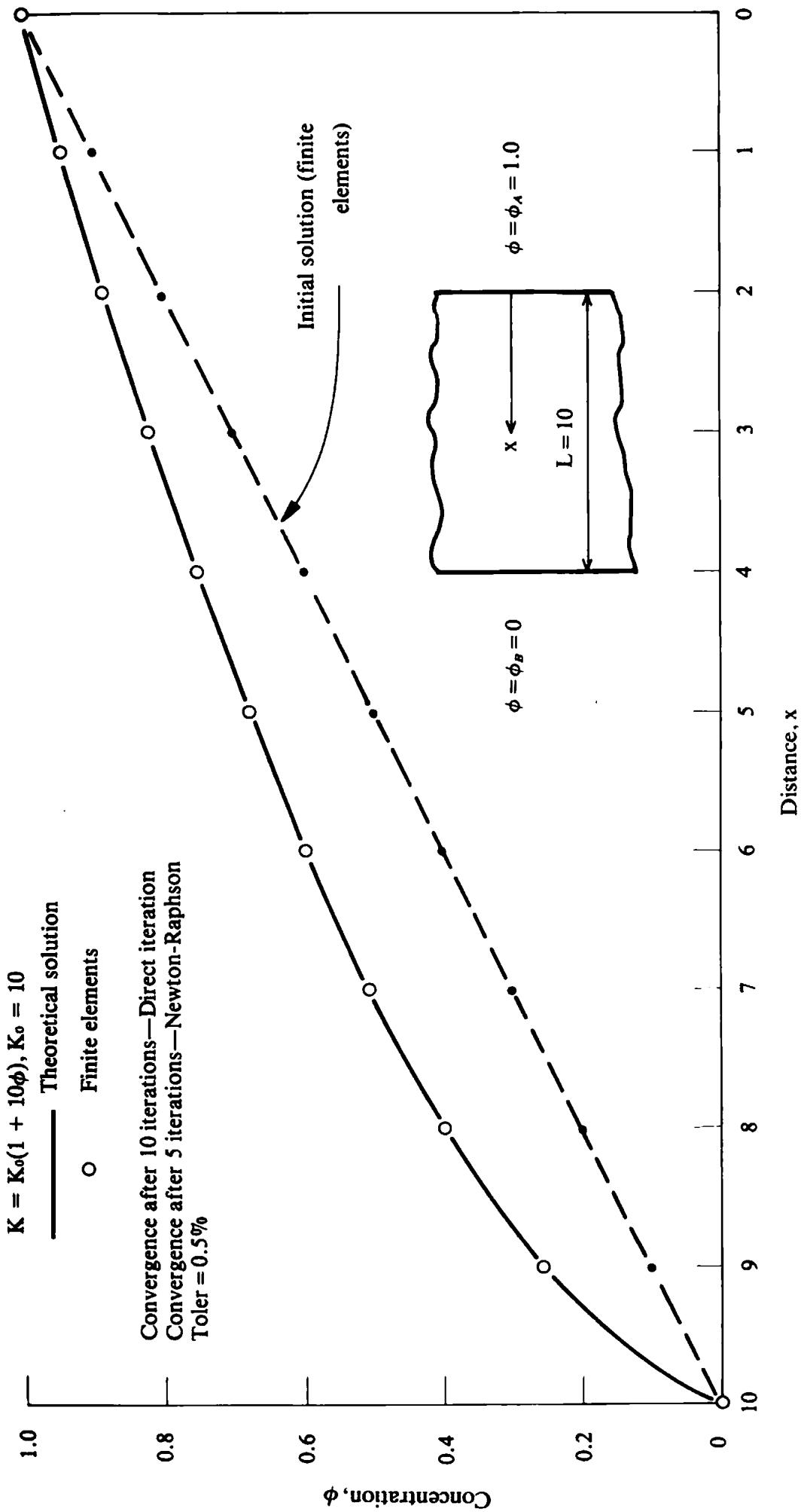# 3.9.3 Numerical examples The first numerical example considered is illustrated in Fig. 3.3. The situation shown could physically represent the diffusion of a gas through a membrane in which case $\phi$ is the gas concentration and K is the diffusivity of the membrane. Alternatively, the problem also represents the conduction of heat through a one-dimensional solid in which case $\phi$ is the temperature and K the thermal conductivity. The boundary conditions assumed are 

line

| Distance, x | Theoretical solution (φ) | Finite elements (φ) | | ----------- | ------------------------ | ------------------- | | 10 | 0.0 | 0.0 | | 9 | 0.25 | 0.25 | | 8 | 0.4 | 0.4 | | 7 | 0.5 | 0.5 | | 6 | 0.6 | 0.6 | | 5 | 0.7 | 0.7 | | 4 | 0.8 | 0.8 | | 3 | 0.9 | 0.9 | | 2 | 0.95 | 0.95 | | 1 | 0.98 | 0.98 | | 0 | 1.0 | 1.0 |

Fig. 3.3 Quasi-harmonic equation example—Problem of gas diffusion through a permeable membrane. specified values of the unknown at the two boundaries. The term K is assumed to vary with the unknown $\phi$ according to $$ K = K _ {0} (1 + 1 0 \phi) = K _ {0} (1 + g (\phi)). \tag {3.22} $$ An analytical solution $^{(6)}$ exists for this problem which enables $\phi$ to be determined from $$ \frac {\phi_ {A} + F \left(\phi_ {A}\right) - \phi - F (\phi)}{\phi_ {A} + F \left(\phi_ {A}\right) - \phi_ {B} - F \left(\phi_ {B}\right)} = \frac {x}{L}, \tag {3.23} $$ where $$ F (\phi) = \int_ {0} ^ {\phi} g \left(\phi^ {\prime}\right) d \phi^ {\prime}. \tag {3.24} $$ In the present case, $g(\phi) = 10\phi$ which gives on substitution in (3.24) and then in (3.23) $$ \frac {6 - \phi - 5 \phi^ {2}}{6} = \frac {x}{1 0}, \tag {3.25} $$ which allows $\phi$ to be determined for any value of $x$ and is shown as the full line in Fig. 3.3. The initial finite element solution (i.e., after the first iteration) is shown in Fig. 3.3 as the broken line and, as expected, is linear. The results upon convergence, after 10 iterations, of the process are then included as circles and it is seen that the numerical solution coincides with the theoretical values. For example, for $x = 6$ , the theoretical solution is $\phi = 0\cdot 6$ , whilst the finite element analysis yields $\phi = 0\cdot 599999$ (see Appendix IV). 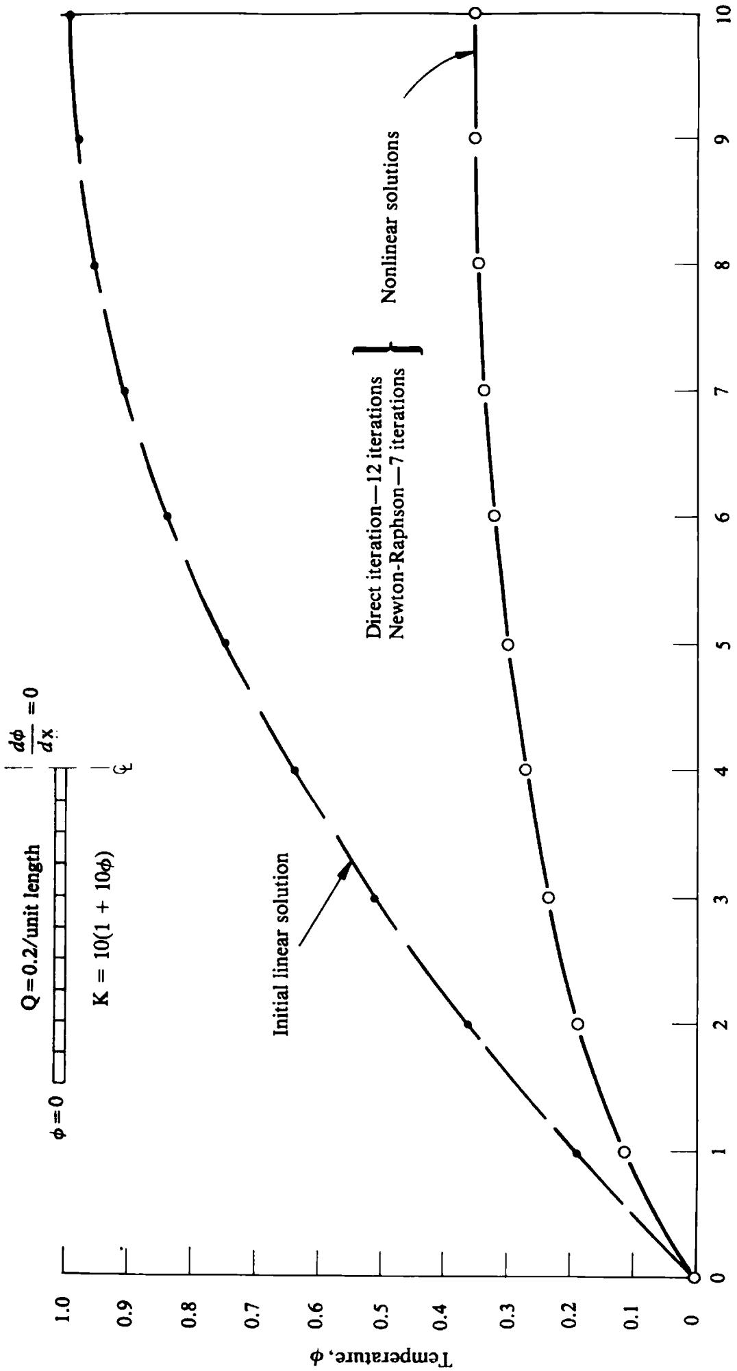The second example considered includes the effect of the term Q in (2.15). For thermal problems this can be physically interpreted as a heat generation/unit length and must be specified as a loading, according to (2.26), in subroutine DATA. Figure 3.4 shows the problem to be considered. A bar with its surface insulated generates heat internally and the temperature at its ends is maintained at zero value. Due to symmetry only one half of the problem is analysed with the symmetry condition $d\phi/dx = 0$ at the centreline being invoked. The initial solution corresponding to $K = K_{0}$ is shown and is practically identical to the theoretical value. The process converged to the nonlinear solution after 12 iterations with the temperature being markedly reduced. The reduction is greater in regions of higher initial temperature due to the comparatively greater increase in material ‘stiffness’ in these areas. # 3.10 Program for the solution of one-dimensional quasi-harmonic problems by the Newton-Raphson method As seen in Section 2.3, use of this method results in the assembled stiffness equations being nonsymmetric. The equation assembly and solution routines developed in Section 3.4 made no use of the symmetry properties of the 

line

| Iteration | Initial linear solution | Direct iteration—12 iterations Newton-Raphson—7 iterations | Nonlinear solutions | | --------- | ------------------------ | ------------------------------------------------------------- | ------------------- | | 0 | 0.0 | 0.0 | 0.0 | | 1 | 0.19 | 0.11 | 0.11 | | 2 | 0.36 | 0.19 | 0.19 | | 3 | 0.51 | 0.23 | 0.23 | | 4 | 0.63 | 0.27 | 0.27 | | 5 | 0.74 | 0.30 | 0.30 | | 6 | 0.83 | 0.32 | 0.32 | | 7 | 0.90 | 0.34 | 0.34 | | 8 | 0.95 | 0.35 | 0.35 | | 9 | 0.98 | 0.35 | 0.35 | | 10 | 1.0 | 0.35 | 0.35 |

Fig. 3.4 Quasi-harmonic equation example—Heat generation in an axial bar. stiffness matrices. They are therefore applicable to this method of analysis without modification. Three additional subroutines need to be developed. These are the element stiffness subroutine ASTIF1 and, since solution convergence is now based on the elimination of the residual forces, subroutine REFOR1 must be formed to calculate these forces and subroutine CONVER to monitor their convergence to zero. The master segment controlling the solution process is again that developed in Section 3.8 and the remaining subroutines accessed by this segment have also been described previously. # 3.10.1 Element stiffness formulation subroutine, ASTIF1 For solution by the Newton–Raphson process, the ‘stiffness’ equations which require solution are summarised in (2.12) where it is seen that the total stiffness is the sum of symmetric, H, and nonsymmetric, $H'$ , contributions. The symmetric stiffness matrix is given by (2.25) and the nonsymmetric terms depend on the particular form of material nonlinearity. For a material nonlinearity of the form (2.27), the nonsymmetric portion of the stiffness matrix is given by (2.29). The subroutine which evaluates and sums these separate contributions is now presented below. ```txt SUBROUTINE ASTIF1 ASTF 1 C************************** ASTF 2 C ASTF 3 C *** CALCULATES ELEMENT STIFFNESS MATRICES ASTF 4 C ASTF 5 C************************** ASTF 6 COMMON/UNIM1/NPOIN.NELEM,NBOUN,NLOAD,NPROP,NNODE,IINCS,IITER, ASTF 7 . KRESL,NCHEK,TOLER,NALGO.NSVAB,NDOFN,NINCS,NEVAB, ASTF 8 . NITER.NOUTP,FACTO,PVALU ASTF 9 COMMON/UNIM2/PROPS(5.4),COORD(26),LNODS(25,2),IFPRE(52), ASTF 10 . FIXED(52),TLOAD(25,4),RLOAD(25,4),ELOAD(25,4), ASTF 11 . MATNO(25),STRES(25,2),PLAST(25),XDISP(52), ASTF 12 . TDISP(26.2),TREAC(26.2),ASTIF(52,52),ASLOD(52), ASTF 13 . REACT(52),FRESV(1352),PEFIX(52),ESTIF(4.4) ASTF 14 REWIND 1 ASTF 15 DO 10 IELEM=1.NELEM ASTF 16 LPROP=MATNO(IELEM) ASTF 17 STERM=PROPS(LPROP,1) ASTF 18 GRADU=PROPS(LPROP,2) ASTF 19 NODE1=LNODS(IELEM,1) ASTF 20 NODE2=LNODS(IELEM,2) ASTF 21 ELENG=ABS(COORD(NODE1)-COORD(NODE2)) ASTF 22 AVERG=(TDISP(NODE1.1)+TDISP(NODE2,1))/2.0 ASTF 23 FMULT=STERM*VARIA(AVERG)/ELENG ASTF 24 DIFFR=TDISP(NODE1.1)-TDISP(NODE2,1) ASTF 25 COEFF=STERM*GRADU*DIFFR/(2.0*ELENG) ASTF 26 ESTIF(1,1)=FMULT+COEFF ASTF 27 ESTIF(1,2)=-FMULT+COEFF ASTF 28 ESTIF(2,1)=-FMULT-COEFF ASTF 29 ESTIF(2,2)=FMULT-COEFF ASTF 30 WRITE(1) ESTIF ASTF 31 10 CONTINUE ASTF 32 RETURN ASTF 33 END ASTF 34 ```