yielding of the end sections followed by a further reduction when the central section becomes plastic resulting in a beam failure mechanism. # 5.5 Elasto-plastic layered Timoshenko beams # 5.5.1 Yielding of layered beams In the ‘layered’ approach the beam or the plate is subdivided into a chosen number of layers, as shown in Fig. 5.8. 

text_image

(a) Layered beam Layer i


text_image

(b) Layered plate Layer i

Fig. 5.8 Layered subdivision of beam and plate. In the finite element solution it is assumed that as soon as the stress in the middle of the outer layers reaches the yield value, then the outer layers become plastic, while the rest of the layers remain elastic, as shown in  Fig. 5.9 Yielding of layered beam. Fig. 5.9. Then, as plastification propagates, more layers become plastic, until the whole cross-section eventually becomes plastic. # 5.5.2 Formation of the stiffness matrix in the layered approach In the layered approach, we work in terms of stresses and not in terms of stress resultants as in the nonlayered approach. The state of stress at the middle of a layer is taken as representative for the entire layer. Contributions to the stress resultants M and Q are found for each layer separately by integrating over the layer thickness only. The bending moments and shear forces are then found from the contributions of all the layers of the beam element. The displacement field, stress-strain relationship and strain-displacement relationship are given in (5.1)-(5.10). The virtual work expression is given by (5.11) and when we evaluate the bending moment M and shear force Q we use a mid-ordinate rule as follows: $$ M = E I \left(- \frac {d \theta}{d x}\right) \quad \text { and } \quad Q = G \hat {A} \epsilon_ {s} \tag {5.48} $$ where $$ E I = \sum_ {l} E _ {l} b _ {l} z _ {l} ^ {2} t _ {l} \tag {5.49} $$ and $$ G \hat {A} = \sum_ {l} G _ {l} b _ {l} t _ {l} \tag {5.50} $$ and where $b_{l}$ is the layer breadth $t_{l}$ is the layer thickness $z_{l}$ is the $z$ -coordinate at the middle of the layer $E_{l}$ is the Young's modulus of the layer material and $G_{l}$ is the Shear modulus of the layer material. However, if the stress at the middle surface of a layer reaches the uniaxial yield stress of the layer material, the whole layer is considered to be plastic and $E_{l}$ is replaced by $$ E _ {l} \left(1 - \frac {E _ {l}}{E _ {l} + H ^ {\prime}}\right), $$ where $H'$ is the uniaxial strain hardening parameter. As mentioned before, the shear force–shear strain relationship is always elastic. # 5.5.3 Solution of nonlinear equations Recall that the virtual work expression (5.11) has the form $$ \int_ {0} ^ {l} \int_ {- t / 2} ^ {t / 2} \int_ {b (- t / 2)} ^ {b (t / 2)} \left\{- z \frac {d (\delta \theta)}{d x} \sigma_ {x} + \delta \beta \tau_ {x z} \right\} d y d z d x - \int_ {0} ^ {l} \delta w q d x = 0. \tag {5.51} $$ The mid-ordinate rule is again used to evaluate the first two integrals in (5.51) so that we obtain $$ [ \delta \varphi ] ^ {T} [ \boldsymbol {p} _ {f} + \boldsymbol {p} _ {s} ] - [ \delta \varphi ] ^ {T} \boldsymbol {f} = 0 \tag {5.52} $$ where $$ \boldsymbol {p} _ {f} = \int_ {0} ^ {l} [ \boldsymbol {B} _ {f} ] ^ {T} \bar {M} d x $$ and $$ \boldsymbol {p} _ {s} = \int_ {0} ^ {l} [ \boldsymbol {B} _ {s} ] ^ {T} \bar {Q} d x $$ in which $B_{f}$ , $B_{s}$ and $\delta\varphi$ have been defined in (5.40), (5.41) and (5.43) respectively and in which $$ \overline {{{M}}} = \sum_ {l} b _ {l} \sigma_ {x l} z _ {l} t _ {l} \tag {5.53} $$ and $$ \bar {Q} = \sum_ {l} b _ {l} \tau_ {x z l} t _ {l}. \tag {5.54} $$ Note that $\sigma_{xl}$ and $\tau_{xzl}$ are the direct and shear stresses in the layer respectively. Since (5.52) is true for any arbitrary set of virtual displacements then $$ \boldsymbol {p} _ {f} + \boldsymbol {p} _ {s} - \boldsymbol {f} = 0. \tag {5.55} $$ Contributions to $p_{f}$ and $p_{s}$ may be evaluated separately from each element so that $$ \begin{array}{l} \boldsymbol {p} _ {f} ^ {(e)} = \int_ {x _ {1} ^ {(e)}} ^ {x _ {2} ^ {(e)}} [ \boldsymbol {B} _ {f} ^ {(e)} ] ^ {T} \bar {M} ^ {(e)} d x = \int_ {x _ {1} ^ {(e)}} ^ {x _ {2} ^ {(e)}} \left[ 0, \left(\frac {\bar {M}}{l}\right) ^ {(e)}, 0, - \left(\frac {\bar {M}}{l}\right) ^ {(e)} \right] ^ {T} d x \\ = [ 0, \bar {M} ^ {(e)}, 0, - \bar {M} ^ {(e)} ] ^ {T} \tag {5.56} \\ \end{array} $$ and $$ \begin{array}{l} \boldsymbol {p} _ {s} ^ {(e)} = \int_ {x _ {1} ^ {(e)}} ^ {x _ {2} ^ {(e)}} \left[ \boldsymbol {B} _ {s} ^ {(e)} \right] ^ {T} \bar {Q} ^ {(e)} d x = \int_ {x _ {1} ^ {(e)}} ^ {x _ {2} ^ {(e)}} \left[ - \frac {1}{l ^ {(e)}}, - \frac {1}{2}, \frac {1}{l ^ {(e)}}, - \frac {1}{2} \right] ^ {T} \bar {Q} ^ {(e)} d x \\ = \left[ - \bar {Q} ^ {(e)}, - \frac {(\bar {Q} l) ^ {(e)}}{2}, \bar {Q} ^ {(e)}, - \frac {(\bar {Q} l) ^ {(e)}}{2} \right] ^ {T}. \tag {5.57} \\ \end{array} $$ The complete sequence of nonlinear equation solving is very similar to the one adopted in Table 5.1 for the nonlayered beam. Step 5 is now written as: 5. For each element evaluate for each layer $\sigma_{xl}^{(e)}$ and $\tau_{xzl}^{(e)}$ . Check $\sigma_{xl}^{(e)}$ and adjust its value accordingly to account for any plastic behaviour. Evaluate the stress resultants $\bar{M}^{(e)}$ and $\bar{Q}^{(e)}$ and hence evaluate the residual force vector $[\psi^{(e)}]^{i+1} = p^{(e)} - f^{(e)}$ . Assemble $[\psi^{(e)}]^{i+1}$ into the global residual force vector $\psi^{i+1}$ . # 5.5.4 Overall structure of layered beam program TIMLAY The overall structure of the layered beam program is exactly the same as that of the nonlayered beam program given in Fig. 5.5. Subroutine STIFBL replaces STIFFB and subroutine RFORBL replaces REFORB. Subroutine STIFBL calls a further new routine called LAYER. The master routine BEML has minor changes as shown in the next section. # 5.5.5 Modified and new routines Master BEML This routine is almost identical to routine BEAM described earlier. ```txt MASTER BEML LYBM 1 C**************************LYBM 2 C LYBM 3 C *** ELSTO-PLASTIC LAYERED TIMOSHENKO BEAM PROGRAM LYBM 4 C LYBM 5 C**************************LYBM 6 COMMON/UNIM1/NPOIN,NELEM,NBOUN,NLAYR,NPROP,NNODE,IINCS,IITER, LYBM 7 . KRESL,NCHEK,TOLER,NALGO,NSVAB,NDOFN,NINCS,NEVAB, LYBM 8 . NITER,NOUTP,FACTO LYBM 9 COMMON/UNIM2/PROPS(5,25),COORD(26),LNODS(25,2),IFPRE(52), LYBM 10 . FIXED(52),TLOAD(25,4),RLOAD(25,4),ELOAD(25,4), LYBM 11 . MATNO(25),STRES(25,2),PLAST(250),XDISP(52), LYBM 12 . TDISP(26,2),TREAC(26,2),ASTIF(52,52),ASLOD(52), LYBM 13 . REACT(52),FRESV(1352),PEFIX(52),ESTIF(4,4), LYBM 14 . STRSL(250,2) LYBM 15 CALL DATA LYBM 16 CALL INITIAL LYBM 17 DO 30 IINCS=1,NINCS LYBM 18 CALL INCLOD LYBM 19 DO 10 IITER=1,NITER LYBM 20 CALL NONAL LYBM 21 IF(KRESL.EQ.1) CALL STIFBL LYBM 22 CALL ASSEMB LYBM 23 IF(KRESL.EQ.1) CALL GREDUC LYBM 24 ```

IF(KRESL.EQ.2) CALL RESOLV	LYBM	25
CALL BAKSUB	LYBM	26
CALL RFORBL	LYBM	27
CALL CONUND	LYBM	28
IF(NCHEK.EQ.0) GO TO 20	LYBM	29
IF(IITER.EQ.1.AND.NOUTP.EQ.1) CALL RESULT	LYBM	30
IF(NOUTP.EQ.2) CALL RESULT	LYBM	31
10 CONTINUE	LYBM	32
WRITE(6,900)	LYBM	33
900 FORMAT(1H0,5X,'SOLUTION NOT CONVERGED')	LYBM	34
STOP	LYBM	35
20 CALL RESULT	LYBM	36
30 CONTINUE	LYBM	37
STOP	LYBM	38
END	LYBM	39

Subroutine STIFBL This routine calculates the element stiffness matrices for the elasto-plastic layered Timoshenko beam element.

	SUBROUTINE STIFBL	STBL	1
C**********	**********	STBL	2
C		STBL	3
C *** CALCULATES ELEMENT STIFFNESS MATRICES		STBL	4
C		STBL	5
C**********	**********	STBL	6
	COMMON/UNIM1/NPOIN,NELEM,NBOUN,NLAYR,NPROP,NNODE,IINCS,IITER,	STBL	7
	KRESL,NCHEK,TOLER,NALGO,NSVAB,NDOFN,NINCS,NEVAB,	STBL	8
	NITER,NOUTP,FACTO	STBL	9
	COMMON/UNIM2/PROPS(5,25),COORD(26),LNODS(25,2),IFPRE(52),	STBL	10
	FIXED(52),TLOAD(25,4),RLOAD(25,4),ELOAD(25,4),	STBL	11
	MATNO(25),STRES(25,2),PLAST(250),XDISP(52),	STBL	12
	TDISP(26,2),TREAC(26,2),ASTIF(52,52),ASLOD(52),	STBL	13
	REACT(52),FRESV(1352),PEFIX(52),ESTIF(4,4),	STBL	14
	STRSL(250,2)	STBL	15
	REWIND 1	STBL	16
	DO 20 IELEM=1,NELEM	STBL	17
	LPROP=MATNO(IELEM)	STBL	18
	CALL LAYER(IELEM,EIVAL,SVALU)	STBL	19
	HARDS=PROPS(LPROP,4)	STBL	20
	NODE1=LNODS(IELEM,1)	STBL	21
	NODE2=LNODS(IELEM,2)	STBL	22
	ELENG=ABS(COORD(NODE2)-COORD(NODE1))	STBL	23
	VALU1=0.5*SVALU	STBL	24
	VALU2=SVALU/ELENG	STBL	25
	VALU3=EIVAL/ELENG	STBL	26
	VALU4=0.25*SVALU*ELENG	STBL	27
	ESTIF(1,1)=VALU2	STBL	28
	ESTIF(1,2)=VALU1	STBL	29
	ESTIF(1,3)=-VALU2	STBL	30
	ESTIF(1,4)=VALU1	STBL	31
	ESTIF(2,2)=VALU3+VALU4	STBL	32
	ESTIF(2,3)=-VALU1	STBL	33
	ESTIF(2,4)=-VALU3+VALU4	STBL	34
	ESTIF(3,3)=VALU2	STBL	35
	ESTIF(3,4)=-VALU1	STBL	36
	ESTIF(4,4)=VALU3+VALU4	STBL	37
	DO 10 ISTIF=1,4	STBL	38
	DO 10 JSTIF=ISTIF,4	STBL	39
10	ESTIF(JSTIF,ISTIF)=ESTIF(ISTIF,JSTIF)	STBL	40
	WRITE(1) ESTIF	STBL	41
20	CONTINUE	STBL	42
	RETURN	STBL	43
	END	STBL	44

STBL 19 Call routine LAYER which evaluates approximate values of EI and exact values of $GA$ using a mid-ordinate rule. Note that certain layers may be plastic. Subroutine RFORBL This routine evaluates p for the layered beam using the mid-ordinate rule.

SUBROUTINE RFORBL	RFRL	1
C**********	RFRL	2
C	RFRL	3
C *** CALCULATES INTERNAL EQUIVALENT NODAL FORCES	RFRL	4
C	RFRL	5
C**********	RFRL	6
COMMON/UNIM1/NPOIN,NELEM,NBOUN,NLAYR,NPROP,NNODE,IINCS,IITER,	RFRL	7
KRESL,NCHEK,TOLER,NALGO,NSVAB,NDOFN,NINCS,NEVAB,	RFRL	8
NITER,NOUTP,FACTO	RFRL	9
COMMON/UNIM2/PROPS(5,25),COORD(26),LNODS(25,2),IFPRE(52),	RFRL	10
FIXED(52),TLOAD(25,4),RLOAD(25,4),ELOAD(25,4),	RFRL	11
MATNO(25),STRES(25,2),PLAST(250),XDISP(52),	RFRL	12
TDISP(26,2),TREAC(26,2),ASTIF(52,52),ASLOD(52),	RFRL	13
REACT(52),FRESV(1352),PEFIX(52),ESTIF(4,4),	RFRL	14
STRSL(250,2)	RFRL	15
DIMENSION STRAN(2)	RFRL	16
DO 15 IELEM=1,NELEM	RFRL	17
DO 10 IEVAB=1,NEVAB	RFRL	18
10 ELOAD(IELEM,IEVAB)=0.0	RFRL	19
DO 15 IDOFN=1,NDOFN	RFRL	20
15 STRES(IELEM,IDOFN)=0.0	RFRL	21
KLAYR=0	RFRL	22
DO 70 IELEM=1,NELEM	RFRL	23
LPROP=MATNO(IELEM)	RFRL	24
YOUNG=PROPS(LPROP,1)	RFRL	25
SHEAR=PROPS(LPROP,2)	RFRL	26
YIELD=PROPS(LPROP,3)	RFRL	27
HARDS=PROPS(LPROP,4)	RFRL	28
THKTO=PROPS(LPROP,5)	RFRL	29
NODE1=LNODS(IELEM,1)	RFRL	30
NODE2=LNODS(IELEM,2)	RFRL	31
ELENG=ABS(COORD(NODE2)-COORD(NODE1))	RFRL	32
WNOD1=XDISP(NODE1*NDOFN-1)	RFRL	33
WNOD2=XDISP(NODE2*NDOFN-1)	RFRL	34
THTA1=XDISP(NODE1*NDOFN)	RFRL	35
THTA2=XDISP(NODE2*NDOFN)	RFRL	36
STRAN(1)=(THTA1-THTA2)/ELENG	RFRL	37
STRAN(2)=(WNOD2-WNOD1)/ELENG	RFRL	38
-0.5*(THTA1+THTA2)	RFRL	39
ZMIDL=-THKTO/2.0	RFRL	40
KOUNT=5	RFRL	41
DO 50 ILAYR=1,NLAYR	RFRL	42
KLAYR=KLAYR+1	RFRL	43
KOUNT=KOUNT+1	RFRL	44
BRDTH=PROPS(LPROP,KOUNT)	RFRL	45
KOUNT=KOUNT+1	RFRL	46
THICK=PROPS(LPROP,KOUNT)	RFRL	47
ZMIDL=ZMIDL+THICK/2.0	RFRL	48
STLIN=YOUNG*STRAN(1)*ZMIDL	RFRL	49
STCUR=STRSL(KLAYR,1)+STLIN	RFRL	50
PREYS=YIELD+HARDS*ABS(PLAST(KLAYR))	RFRL	51
IF(ABS(STRSL(KLAYR,1)).GE.PREYS) GO TO 20	RFRL	52
ESCUR=ABS(STCUR)-PREYS	RFRL	53
IF(ESCUR.LE.0.0) GO TO 40	RFRL	54

```csv RFACT=ESCUR/ABS(STLIN) RFRL 55 GO TO 30 RFRL 56 20 IF(STRSL(KLAYR,1).GT.0.0.AND.STLIN.LE.0.0) GO TO 40 RFRL 57 IF(STRSL(KLAYR,1).LT.0.0.AND.STLIN.GE.0.0) GO TO 40 RFRL 58 RFACT=1.0 RFRL 59 30 REDUC=1.0-RFACT RFRL 60 STRSL(KLAYR,1)=STRSL(KLAYR,1)+REDUC*STLIN+ RFRL 61 • RFACT*YOUNG*(1.0-YOUNG/(YOUNG+HARDS))*STRAN(1)*ZMIDL RFRL 62 PLAST(KLAYR)=PLAST(KLAYR)+RFACT*STRAN(1)*YOUNG/(YOUNG+HARDS) RFRL 63 .*ZMIDL RFRL 64 GO TO 45 RFRL 65 40 STRSL(KLAYR,1)=STRSL(KLAYR,1)+STLIN RFRL 66 45 STRSL(KLAYR,2)=STRSL(KLAYR,2)+STRAN(2)*SHEAR RFRL 67 STRES(IELEM,1)=STRES(IELEM,1)+STRSL(KLAYR,1)* RFRL 68 • BRDTH*THICK*ZMIDL RFRL 69 STRES(IELEM,2)=STRES(IELEM,2)+STRSL(KLAYR,2)* RFRL 70 • BRDTH*THICK RFRL 71 ZMIDL=ZMIDL+THICK/2.0 RFRL 72 50 CONTINUE RFRL 73 ELOAD(IELEM,1)=ELOAD(IELEM,1)-STRES(IELEM,2) RFRL 74 ELOAD(IELEM,2)=ELOAD(IELEM,2)+STRES(IELEM,1) RFRL 75 • -0.5*ELENG*STRES(IELEM,2) RFRL 76 ELOAD(IELEM,3)=ELOAD(IELEM,3)+STRES(IELEM,2) RFRL 77 ELOAD(IELEM,4)=ELOAD(IELEM,4)-STRES(IELEM,1) RFRL 78 • -0.5*ELENG*STRES(IELEM,2) RFRL 79 70 CONTINUE RFRL 80 RETURN RFRL 81 END RFRL 82 ``` Subroutine LAYER This routine evaluates EI and $GA\hat{A}$ using the mid-ordinate rule. Note that certain layers may be plastic and therefore have a modified E. ```txt SUBROUTINE LAYER(IELEM,EIVAL,SVALU) LAYR 1 C****************************************************************************************** C LAYR 2 C LAYR 3 C *** CALCULATES INTEGRATED VALUES FOR EI AND GA THROUGH DEPTH LAYR 4 C LAYR 5 C****************************************************************************************** COMMON/UNIM1/NPOIN,NELEM,NBOUN,NLAYR,NPROP,NNODE,IINCS,IITER, LAYR 7 . KRESL,NCHEK,TOLER,NALGO,NSVAB,NDOFN,NINCS,NEVAB, LAYR 8 . NITER,NOUTP,FACTO LAYR 9 COMMON/UNIM2/PROPS(5,25),COORD(26),LNODS(25,2),IFPRE(52), LAYR 10 . FIXED(52),TLOAD(25,4),RLOAD(25,4),ELOAD(25,4), LAYR 11 . MATNO(25),STRES(25,2),PLAST(250),XDISP(52), LAYR 12 . TDISP(26,2),TREAC(26,2),ASTIF(52,52),ASLOD(52), LAYR 13 . REACT(52),FRESV(1352),PEFIX(52),ESTIF(4,4), LAYR 14 . STRSL(250,2) LAYR 15 EIVAL=0.0 LAYR 16 SVALU=0.0 LAYR 17 LPROP=MATNO(IELEM) LAYR 18 KLAYR=(IELEM-1)*NLAYR LAYR 19 SHEAR=PROPS(LPROP,2) LAYR 20 HARDS=PROPS(LPROP,4) LAYR 21 THKTO=PROPS(LPROP,5) LAYR 22 ZMIDL=-THKTO/2.0 LAYR 23 KOUNT=5 LAYR 24 DO 10 ILAYR=1,NLAYR LAYR 25 KLAYR=KLAYR+1 LAYR 26 YOUNG=PROPS(LPROP,1) LAYR 27 IF(PLAST(KLAYR).NE.0.0) YOUNG=YOUNG*(1.0-YOUNG/(YOUNG+HARDS)) LAYR 28 ``` KOUNT=KOUNT+1 LAYR 29 BRDTH=PROPS(LPROP,KOUNT) LAYR 30 KOUNT=KOUNT+1 LAYR 31 THICK=PROPS(LPROP,KOUNT) LAYR 32 ZMIDL=ZMIDL+THICK/2.0 LAYR 33 EIVAL=EIVAL+YOUNG*BRDTH*THICK*ZMIDL*ZMIDL LAYR 34 SVALU=SVALU+SHEAR*BRDTH*THICK LAYR 35 ZMIDL=ZMIDL+THICK/2.0 LAYR 36 10 CONTINUE LAYR 37 RETURN LAYR 38 END LAYR 39 # 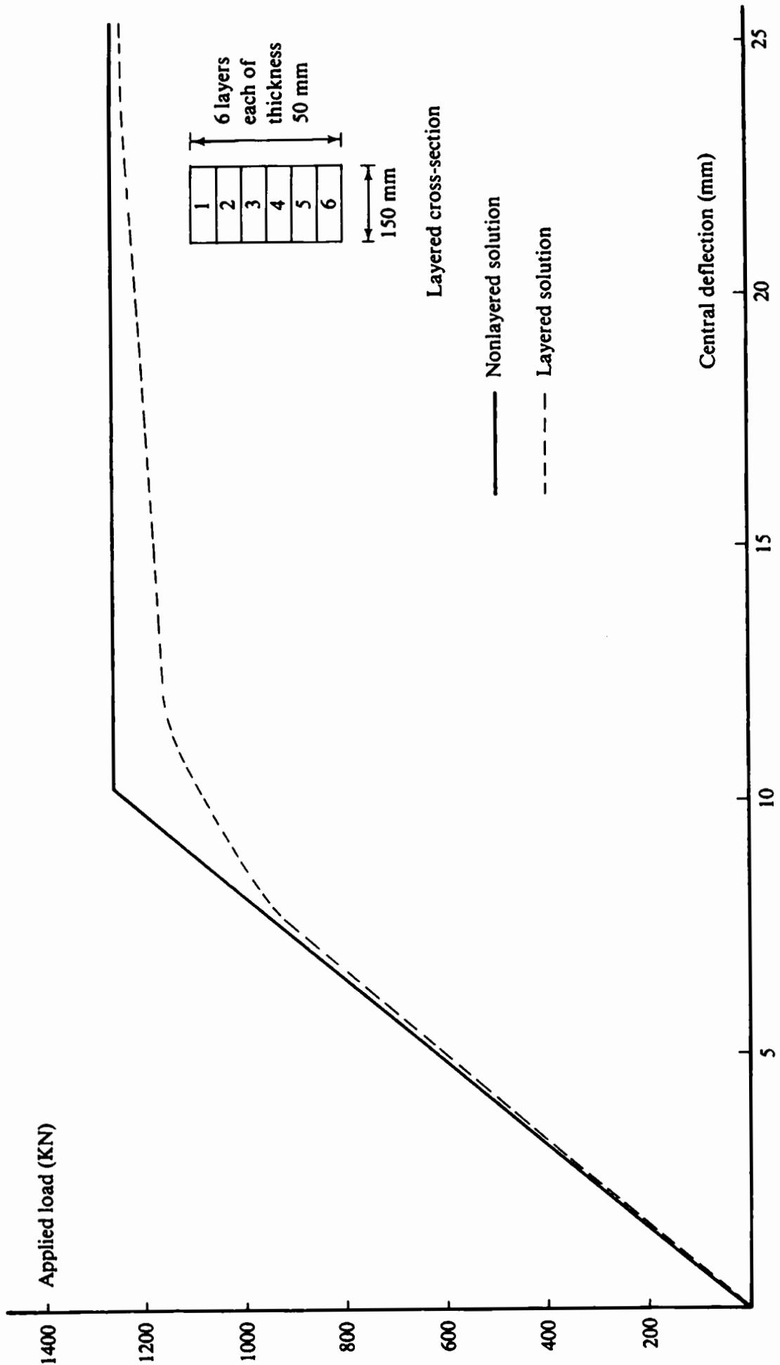5.5.6 Examples of layered elasto-plastic Timoshenko beam analysis The third example considered in this chapter is the elasto-plastic analysis of the simple beam of Example 5.1. The layered solution is adopted in this case. A typical input data listing is provided in Appendix IV. The results for both nonlayered and layered solutions to this beam problem are reproduced in Fig. 5.10. The last example to be considered here is the layered solution of the clamped I-beam given in Example 5.1. Again, both nonlayered and layered solution results are illustrated in Fig. 5.11. From Figs. 5.10 and 5.11 it is obvious that the layered solution is more realistic. Yielding takes place gradually through the layers, resulting in smoother curves representing the load-displacement relationship. # 5.6 Problems 5.1 Derive the main expressions for the elasto-plastic analysis of Timoshenko beams using elements with (i) Quadratic shape functions $$ N _ {1} ^ {(e)} = \frac {(x ^ {(e)} - x _ {2} ^ {(e)}) (x ^ {(e)} - x _ {3} ^ {(e)})}{(x _ {1} ^ {(e)} - x _ {2} ^ {(e)}) (x _ {1} ^ {(e)} - x _ {3} ^ {(e)})} $$ $$ N _ {2} ^ {(e)} = \frac {\big (x ^ {(e)} - x _ {1} ^ {(e)} \big) \big (x ^ {(e)} - x _ {3} ^ {(e)} \big)}{\big (x _ {2} ^ {(e)} - x _ {1} ^ {(e)} \big) \big (x _ {2} ^ {(e)} - x _ {3} ^ {(e)} \big)} $$ $$ N _ {3} ^ {(e)} = \frac {\left(x ^ {(e)} - x _ {1} ^ {(e)}\right) \left(x ^ {(e)} - x _ {2} ^ {(e)}\right)}{\left(x _ {3} ^ {(e)} - x _ {1} ^ {(e)}\right) \left(x _ {3} ^ {(e)} - x _ {2} ^ {(e)}\right)} \tag {5.58} $$ 

line

| Central deflection (mm) | Nonlayered solution (KN) | Layered solution (KN) | | ----------------------- | ------------------------ | --------------------- | | 0 | 0 | 0 | | 5 | 600 | 550 | | 10 | 1250 | 1150 | | 15 | 1275 | 1200 | | 20 | 1280 | 1230 | | 25 | 1285 | 1250 |

Fig. 5.10 Load-deflection diagrams for simply supported beam. 

line

| Layer number | Cross-section (mm) | Applied load intensity (KN/mm) | | ------------ | ------------------- | ------------------------------ | | 2 | 200 | 0.45 | | 3 | 200 | 0.44 | | 4 | 200 | 0.43 | | 5 | 200 | 0.42 | | 6 | 200 | 0.41 |