# 7.9 Numerical examples
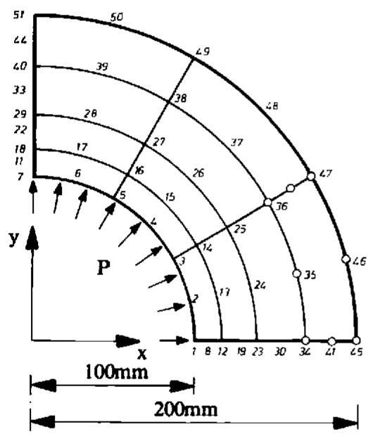
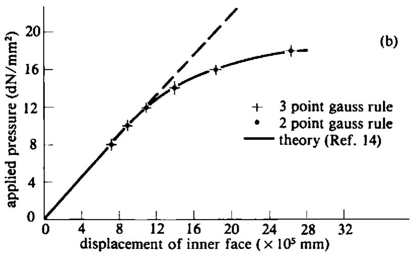
The first numerical example considered is illustrated in Fig. 7.12(a). The problem studied is that of a thick cylinder subjected to a gradually increasing internal pressure, with plane strain conditions being assumed in the axial direction. A Von Mises yield criterion is assumed and the numerical solutions obtained compared with the theoretical results of Reference 14. The pressure/radial displacement characteristics are shown in Fig. 7.12(b) and good
radar
| Angle (°) | Value |
| --------- | ----- |
| 40 | 50 |
| 45 | 50 |
| 50 | 50 |
| 55 | 50 |
| 60 | 50 |
| 65 | 50 |
| 70 | 50 |
| 75 | 50 |
| 80 | 50 |
| 85 | 50 |
| 90 | 50 |
| 95 | 50 |
| 100 | 50 |
| 105 | 50 |
| 110 | 50 |
| 115 | 50 |
| 120 | 50 |
| 125 | 50 |
| 130 | 50 |
| 135 | 50 |
| 140 | 50 |
| 145 | 50 |
| 150 | 50 |
| 155 | 50 |
| 160 | 50 |
| 165 | 50 |
| 170 | 50 |
| 175 | 50 |
| 180 | 50 |
| 185 | 50 |
| 190 | 50 |
| 195 | 50 |
| 200 | 50 |
| 205 | 50 |
| 210 | 50 |
| 215 | 50 |
| 220 | 50 |
| 225 | 50 |
| 230 | 50 |
| 235 | 50 |
| 240 | 50 |
| 245 | 50 |
| 250 | 50 |
| 255 | 50 |
| 260 | 50 |
| 265 | 50 |
| 270 | 50 |
| 275 | 50 |
| 280 | 50 |
| 285 | 50 |
| 290 | 50 |
| 295 | 50 |
| 300 | 50 |
| 305 | 50 |
| 310 | 50 |
| 315 | 50 |
| 320 | 50 |
| 325 | 50 |
| 330 | 50 |
| 335 | 50 |
| 340 | 50 |
| 345 | 50 |
| 350 | 50 |
| 355 | 50 |
| 360 | 50 |
| 365 | 50 |
| 370 | 50 |
| 375 | 50 |
| 380 | 50 |
| 385 | 50 |
| 390 | 50 |
| 395 | 50 |
| 400 | 50 |
| 405 | 50 |
| 410 | 50 |
| 415 | 50 |
| 420 | 50 |
| 425 | 50 |
| 430 | 50 |
| 435 | 50 |
| 440 | 50 |
| 445 | 50 |
| 450 | 50 |
| 455 | 50 |
| 460 | 50 |
| 465 | 50 |
| 470 | 50 |
| 475 | 50 |
| 480 | 50 |
| 485 | 50 |
| 490 | 50 |
| 495 | 50 |
| 500 | 50 |
| 505 | 50 |
| 510 | 50 |
| 515 | 50 |
| 520 | 50 |
| 525 | 50 |
| 530 | 50 |
| 535 | 50 |
| 540 | 50 |
| 545 | 50 |
| 550 | 50 |
| 555 | 50 |
| 560 | 50 |
| 565 | 50 |
| 570 | 50 |
| 575 | 50 |
| 580 | 50 |
| 585 | 50 |
| 590 | 50 |
| 595 | 50 |
| 600 | 50 |
| 605 | 50 |
| 610 | 50 |
| 615 | 50 |
| 620 | 50 |
| 625 | 50 |
| 630 | 50 |
| 635 | 50 |
| 640 | 50 |
| 645 | 50 |
| 650 | 50 |
| 655 | 50 |
| 660 | 50 |
| 665 | 50 |
| 670 | 50 |
| 675 | 50 |
| 680 | 50 |
| 685 | 50 |
| 690 | 50 |
| 695 | 50 |
| 700 | 50 |
| 705 | 50 |
| 710 | 50 |
| 715 | 50 |
| 720 | 50 |
| 725 | 50 |
| 730 | 50 |
| 735 | 50 |
| 740 | 50 |
| 745 | 50 |
| 750 | 50 |
| 755 | 50 |
| 760 | 50 |
| 765 | 50 |
| 770 | 50 |
| 775 | 50 |
| 780 | 50 |
| 785 | 50 |
| 790 | 50 |
| 795 | 50 |
| 800 | 50 |
| 805 | 50 |
| 810 | 50 |
| 815 | 50 |
| 820 | 50 |
| 825 | 50 |
| 830 | 50 |
| 835 | 50 |
| 840 | 50 |
| 845 | 50 |
| 850 | 50 |
| 855 | 50 |
| 860 | 50 |
| 865 | 50 |
| 870 | 50 |
| 875 | 50 |
| 880 | 50 |
| 885 | 50 |
| 890 | 50 |
| 895 | 50 |
| 900 | 50 |
| 905 | 50 |
| 910 | 50 |
| 915 | 50 |
| 920 | 50 |
| 925 | 50 |
| 930 | 50 |
| 935 | 50 |
| 940 | 50 |
| 945 | 50 |
| 950 | 50 |
| 955 | 50 |
| 960 | 50 |
| 965 | 50 |
| 970 | 50 |
| 975 | 50 |
| 980 | 50 |
| 985 | 50 |
| 990 | 50 |
| 995 | 50 |
| 1000 | 50 |
Elastic modulus, $E = 2.1 \times 10^{4} \, dN/mm^{2}$
Poissons ratio, $\nu = 0.3$
Uniaxial yield stress, $\sigma_{r}=24.0\ dN/mm^{2}$
Strain hardening parameter, $\mathbf{H}' = 00$
Von mises yield criterion
(a)
line
| displacement of inner face (× 10⁵ mm) | 3 point gauss rule | 2 point gauss rule | theory (Ref. 14) |
| ------------------------------------ | ------------------ | ------------------ | ---------------- |
| 0 | 0 | 0 | 0 |
| 8 | 8 | 8 | 8 |
| 12 | 12 | 12 | 12 |
| 16 | 16 | 16 | 16 |
| 20 | 18 | 18 | 18 |
| 24 | 19 | 19 | 19 |
| 28 | 19 | 19 | 19 |
Fig. 7.12 (a) Mesh and material properties employed in the elasto-plastic analysis of an internally pressurised thick cylinder under plane strain conditions. (b) Displacement of the inner surface with increasing pressure for the problem of Fig. 7.12(a).
agreement between the numerical and analytical solutions is evident. In the numerical studies, collapse was deemed to have occurred if the iterative procedure diverged for an incremental load increase.
line
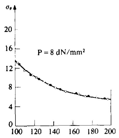
| x | σθ |
| --- | --- |
| 100 | 13 |
| 110 | 12 |
| 120 | 11 |
| 130 | 10 |
| 140 | 9 |
| 150 | 8 |
| 160 | 7 |
| 170 | 6.5 |
| 180 | 6 |
| 190 | 5.5 |
| 200 | 5 |
line
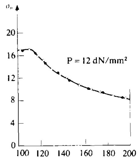
| x | σₙ |
| ---- | --- |
| 100 | 16 |
| 120 | 15 |
| 140 | 13 |
| 160 | 11 |
| 180 | 9 |
| 200 | 8 |
line
| x | σ_e |
| ---- | ---- |
| 100 | 13 |
| 110 | 16 |
| 120 | 19 |
| 130 | 18 |
| 140 | 16 |
| 150 | 14 |
| 160 | 12 |
| 170 | 11 |
| 180 | 10 |
| 190 | 9 |
| 200 | 8 |
line
| x | σθ |
| ---- | ---- |
| 100 | 10 |
| 120 | 15 |
| 140 | 20 |
| 160 | 22 |
| 180 | 20 |
| 200 | 18 |
text_image
Two rows of circular symbols, likely representing data points or indicators, with dots inside each row.
text_image
P 2 3 4 5 6 7 8 9 10
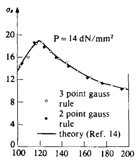
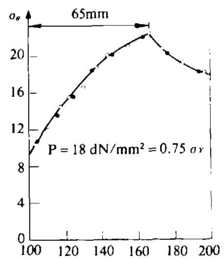
Fig. 7.13 Hoop stress distributions at various pressure values for the problem of Fig. 7.12(a).
Fig. 7.13 shows the circumferential (hoop) stress distributions for specified pressure values. Again a good agreement is evident. In solution both a two-point and three-point Gaussian integration rule was considered. Whilst the nodal displacements obtained by use of both rules are practically identical, it is seen from Fig. 7.13 that use of a $2 \times 2$ integrating rule gives superior stress values to a $3 \times 3$ rule. This is a general result for elasto-plastic problems and therefore use of a two-point rule is recommended. This phenomenon is an example of the benefit of a reduced integration order for parabolic isoparametric elements. $^{(15)}$
line
| Central deflection, w | Intensity of UDL, P |
| --------------------- | ------------------- |
| 0.00 | 0 |
| 0.05 | 100 |
| 0.10 | 150 |
| 0.15 | 200 |
| 0.20 | 250 |
| 0.25 | 275 |
| 0.30 | 280 |
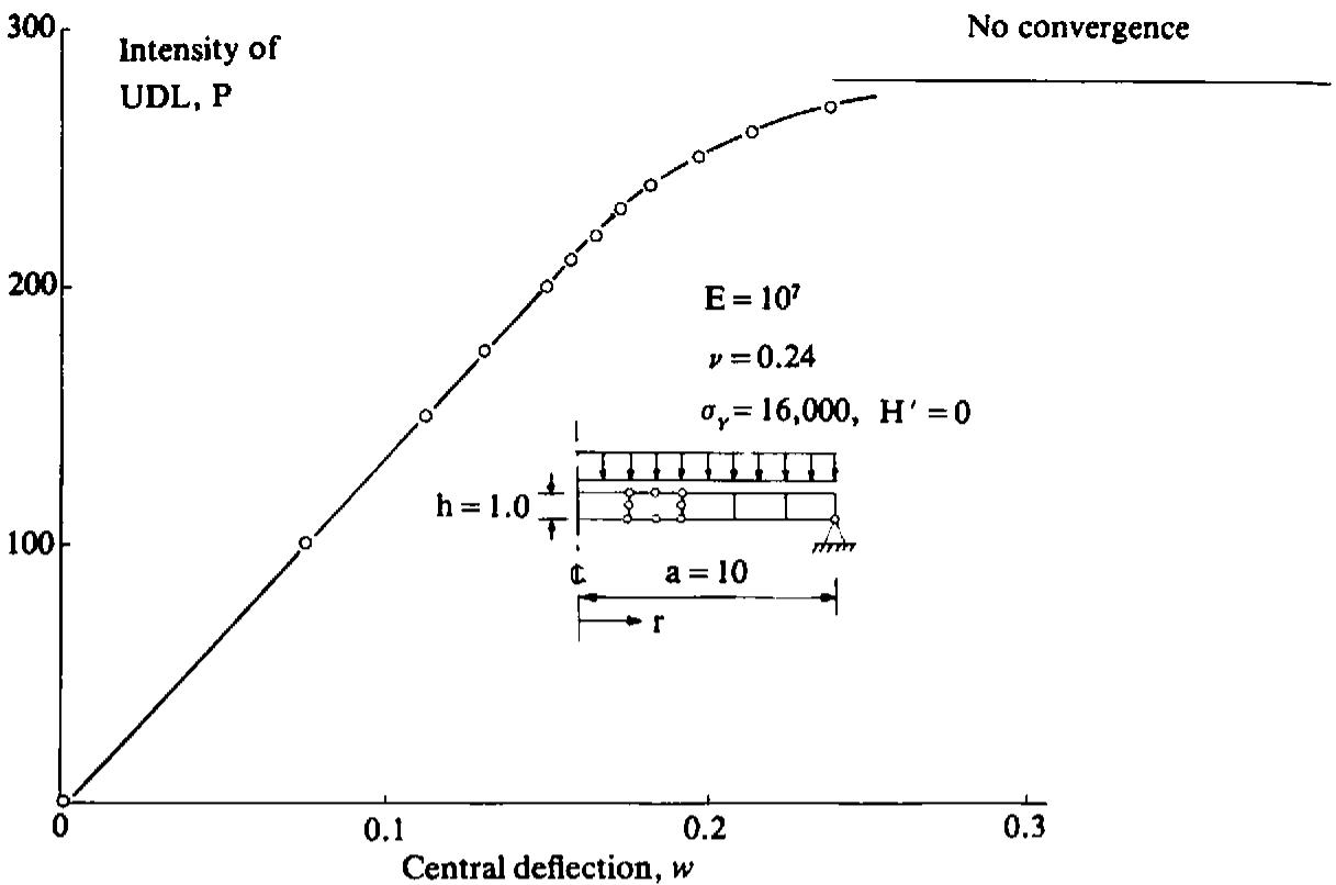
Fig. 7.14 Load/central deflection response for a uniformly loaded simply supported circular plate.
The second example considered is the simply supported circular plate shown in Fig. 7.14.
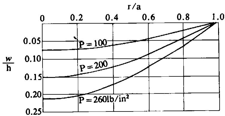
The plate is modelled by five axisymmetric elements and the loading takes the form of a progressively increasing uniformly distributed load. The growth in central deflection with increasing load is shown in Fig. 7.14. A converged solution was obtained for P = 270 but the numerical process diverged for P = 280 and consequently the collapse load is taken to be 270. This is in good agreement with the value of 260 quoted in Ref. 16, particularly in view of the coarse mesh employed in the present study. Fig. 7.15 shows the deflection profile with increasing applied load.
line
| r/a | w/h (P = 100) | w/h (P = 200) | w/h (P = 260 lb/in²) |
| --- | --- | --- | --- |
| 0.0 | 0.05 | 0.15 | 0.20 |
| 0.2 | 0.05 | 0.15 | 0.20 |
| 0.4 | 0.05 | 0.15 | 0.20 |
| 0.6 | 0.05 | 0.15 | 0.20 |
| 0.8 | 0.05 | 0.15 | 0.20 |
| 1.0 | 0.05 | 0.15 | 0.20 |
Fig. 7.15 Deflection profiles for the problem of Fig. 7.14 at various applied load values.
# 7.10 Problems
7.1 In Section 7.2.1 it was stated that the Von Mises law implies that yielding begins when the (recoverable) elastic energy of distortion, $D$ , reaches a critical value. Prove this by showing that $J_2'$ is proportional to $D$ , since $D$ can be written as
$$
D = \frac {1}{2} \sigma_ {i j} \epsilon_ {i j} - \frac {(1 - 2 \nu)}{1 2 \mu (1 + \nu)} (\sigma_ {i i}) ^ {2}. \tag {7.98}
$$
text_image
σ₃
S
√3P₁
0
σ₂
σ₁
√3P₀
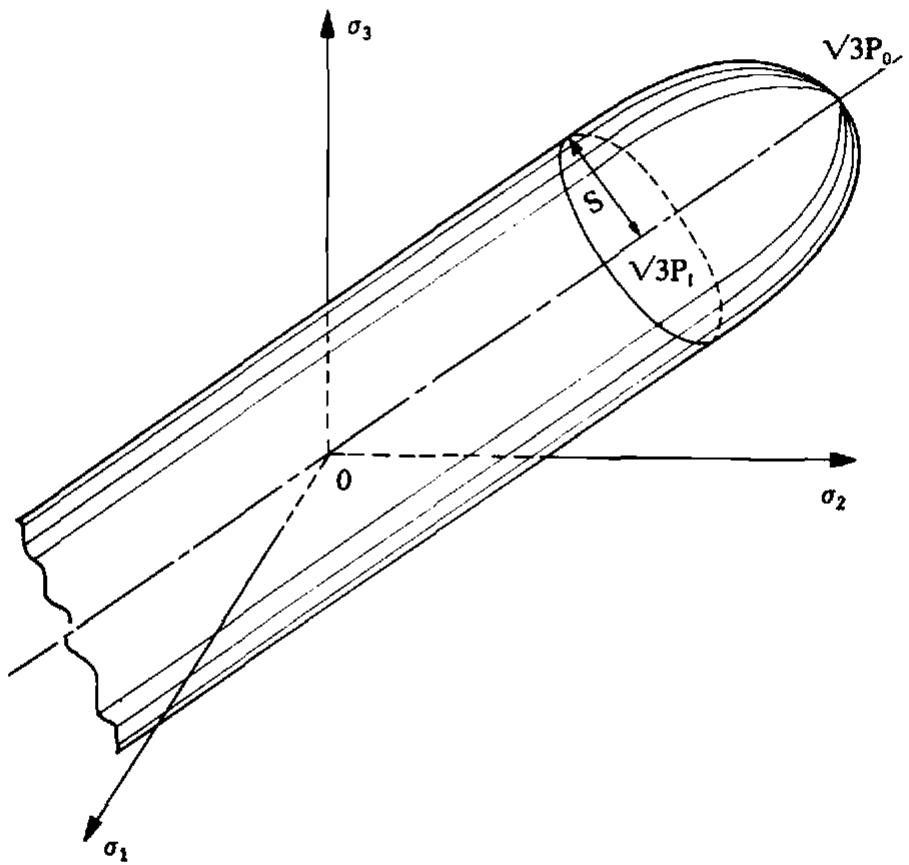
Fig. 7.16 Geometric representation of the Berg yield criterion—Problem 7.2.
7.2 A yield criterion has been proposed by Berg $^{(17)}$ which attempts to account for the tensile failure of a material due to the formation of voids at a sufficiently high strain level. The yield surface is illustrated in Fig. 7.16 and can be seen to be made up of two distinct portions. For stress levels below a mean hydrostatic tension of $P_{I}$ the material yields according to the Von Mises cylinder of radius S. The yield surface in the tensile range is terminated by an elliptic cap whose extremity is defined by $P_{0}$ . The three constants S, $P_{I}$ and $P_{0}$ are material constants and must be experimentally determined. The two distinct portions of the yield surface can be expressed as
$$
\sqrt {2} (J _ {2} ^ {\prime}) ^ {\ddagger} = S \quad \text { for } \sigma_ {m} \leqslant P _ {I}
$$
$$
[ 2 J _ {2} ^ {\prime} + H (\sigma_ {m} - P _ {I}) ^ {2} ] ^ {\frac {1}{2}} = S \quad P _ {I} \leqslant \sigma_ {m} \leqslant P _ {0}, \tag {7.99}
$$
where $H = S^2 / (P_I - P_0)^2$ and $\sigma_m$ is the mean hydrostatic pressure.
Show that this yield criterion can be expressed in the form of three constants $C_{1}$ , $C_{2}$ and $C_{3}$ as indicated in Section 7.4 where
$$
C _ {1} = 0, \quad C _ {2} = \sqrt {2}, \quad C _ {3} = 0 \quad \text { for } \quad \sigma_ {m} \leqslant P _ {I}
$$
$$
C _ {1} = H \left(\sigma_ {m} - P _ {I}\right) / S, \quad C _ {2} = 2 J _ {2} ^ {\prime} / S, \quad C _ {3} = 0 \quad P _ {I} \leqslant \sigma_ {m} \leqslant P _ {0}.
$$
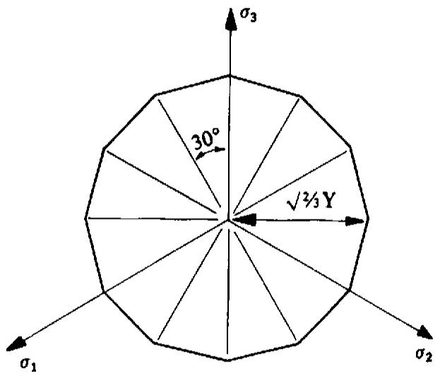
7.3 A certain material yields when the maximum principal stress reaches a critical value, Y. Assuming identical behaviour in tension and compression, determine the geometrical form of the yield surface. The solution is given in Fig. 7.17.
text_image
σ₃
30°
√2/3 Y
σ₁
σ₂
Fig. 7.17 $\pi$ plane representation of a yield criterion based on maximum principal stress values—Problem 7.3.
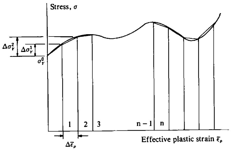
7.4 The assumption of a linear strain hardening material law may prove to be inadequate for certain situations. If the uniaxial stress/strain test curve for the material is known, then it is possible to represent the stress-plastic strain relationship in a piecewise linear fashion as shown in Fig. 7.18 and the instantaneous yield stress can be written in the form $\sigma_{Y} = \sigma_{Y^{0}} + S(\bar{\epsilon}_{p})$ where $S(\bar{\epsilon}_{p})$ is the piecewise linear function describing the increase (or decrease) in the initial yield stress $\sigma_{Y^{0}}$ with the increase of effective plastic strain $\bar{\epsilon}_{p}$ . The program modifications required to describe this behaviour will all be included in subroutine RESIDU, except for changes in material property specification which will need to be made in subroutine INPUT. Carry out all necessary modifications.
line
| Effective plastic strain ε̅p | Stress, σ |
| --------------------------- | --------- |
| Δε̅p (1) | σ⁰_γ |
| Δε̅p (2) | σ²_γ |
| n-1 (3) | σ²_γ |
| n (n) | σ²_γ |
Fig. 7.18 Piecewise-linear representation of material strain hardening—Problem 7.4.
7.5 By using the mesh of Fig. 7.12(a) and solving as an axisymmetric problem, use program PLANET (documented in Appendix II, Section A2.1) to determine the elasto-plastic stress and displacement distributions in a sphere when it is loaded by an incrementally applied internal pressure. The dimensions and material properties of the sphere are given by reference to Fig. 7.12. Assume a Tresca yield criterion for solution and compare your results with the solution given in Ref. 1.
7.6 Use program PLANET to solve the problem illustrated in Fig. 1.2, Chapter 1. Use both a Tresca and Von Mises yield criterion and compare the plastic zone distributions obtained with those of Fig. 1.2.
7.7 Subroutine CONVER, described in Section 6.5.4, bases convergence of the nonlinear solution process on the global norm of the residual force vector. Modify subroutine CONVER so that convergence is based on expression (3.27) in which the summation signs are absent; so that convergence is monitored locally at each of the nodes 1 to N in turn.
7.8 Modify subroutine CONVER, Section 6.5.4 so that convergence is monitored locally at each node according to the displacement changes that occur during a particular iteration, r, as follows.
$$
\frac {| \Delta d ^ {r} |}{| d ^ {1} |} \times 1 0 0 \leqslant \text { TOLER }, \tag {7.100}
$$
where $d^{1}$ is the elastic displacement occurring upon application of the load increment and $\Delta d^{r}$ is the change in nodal displacement during the $r^{th}$ iteration.
7.9 Modify program PLANET to undertake the elasto-plastic solution of three-dimensional solids. To simplify the task consider only the Von Mises yield criterion and assume that the solid is loaded by nodal point loads only.
7.10 The yield criterion to be employed in program PLANET is specified by means of control parameter NCRIT in subroutine INPUT described in Section 6.5.1. In some applications, such as steel-concrete composites, it is necessary to employ a different yield surface for different parts of the structure. Modify program PLANET so that the yield criterion governing elasto-plastic behaviour is separately specified for each element in the solid.
# 7.11 References
1. HILL, R., The Mathematical Theory of Plasticity, Oxford University Press, 1950.
2. PRAGER, W., An Introduction to Plasticity, Addison-Wesley, Amsterdam and London, 1959.
3. HOFFMAN, O. and SACHS, G., Introduction to the Theory of Plasticity for Engineers, McGraw-Hill, 1953.
4. BRIDGMAN, P. W., Studies in Large Plastic Flow and Fracture, McGraw-Hill, New York, 1952.
5. BISHOP, A. W., The strength of soils as engineering materials, Geotechnique, 16, 89–130 (1966).
6. DAVIS, E. M., Theories of plasticity and the failure of soil masses, Ch. 6 Soil Mechanics, Ed. I. K. Lee, Butterworths, London, 1968.
7. ZIENKIEWICZ, O. C., VALLIAPPAN, S. and KING, I. P., Elasto-plastic solutions of engineering problems; Initial stress finite element approach, Int. J. Num. Meth. Engng. 1, 75–100 (1969).
8. YAMADA, Y., YOSHIMURA, N. and SAKURAI, T., Plastic stress-strain matrix and its application for the solution of elastic-plastic problems by Finite Element Method, Int. J. Mech. Sci. 10, 343–354 (1968).
9. BLAND, D. R., The associated flow rule of plasticity, J. Mech. Phy. of Solids, 6, 71–78 (1957).
10. NAYAK, G. C. and ZIENKIEWICZ, O. C., Convenient form of stress invariants for Plasticity, Journ. of the Struct. Div. Proc. of A.S.C.E., 949-953, April 1972.
11. FREDERICK, D. and CHANG, T. S., Continuum Mechanics, Allyn and Bacon, 1965.
12. KOITER, W. T., Stress-strain relations, uniqueness and variational theorems for elastic-plastic materials with singular yield surface, Quart. Appl. Math., 11, 350–354 (1953).
13. HINTON, E. and OWEN, D. R. J., Finite Element Programming, Academic Press, London, 1977.
14. HODGE, P. G. and WHITE, G. N., A quantitative comparison of flow and deformation theories of plasticity' J. Appl. Mech. 17, 180–184 (1950).
15. ZIENKIEWICZ, O. C. and HINTON, E., Reduced integration, function smoothing and non-conformity in finite element analysis (with special reference to thick plates), J. of the Franklin Institute, 302, Nos. 5 and 6, Nov./Dec. 1976.
16. ARMEN, H., Jr., PIFKO, A. and LEVINE, H. S., Finite element analysis of structures in the plastic range, N.A.S.A. Contractor Report, CR.1649 (1971).
17. BERG, C. A., Plastic dilation and void interaction, Battelle Inst. Material Science Colloquia, Sept. 1969. Inelastic Behaviour of Solids, Ed. M. F. Kanninen et al., McGraw-Hill, 171–210, 1970.
18. KRIEG, R. D. and KRIEG, D. B., Accuracies of numerical solution methods for the elastic-perfectly plastic mode, Trans. ASME, J. Pressure Vessel Technology, 99, 4, 510–515 (1977).
19. SCHREYER, H. L., KULAK, R. F. and KRAMER, J. M., Accurate numerical solutions for elastic-plastic models, Trans. ASME, J. Pressure Vessel Technology, 101, 3, 226–234 (1979).
20. SAMUELSSON, A. and FRÖIER, M., Finite elements in plasticity—A variational inequality approach, in The Mathematics of Finite Elements and Applications III, Ed. J. R. Whiteman, Academic Press, 1979.