line
| Overlay | Time (days) | Experimental Strain (%) | Finite element Strain (%) |
| ------- | ----------- | ------------------------ | -------------------------- |
| 1 | 0 | 1.0 | 1.2 |
| 1 | 10 | 1.6 | 1.8 |
| 1 | 20 | 2.0 | 2.2 |
| 1 | 30 | 2.4 | 2.6 |
| 1 | 40 | 2.6 | 2.8 |
| 1 | 50 | 2.8 | 3.0 |
| 1 | 60 | 3.0 | 3.2 |
| 2 | 0 | 1.0 | 1.2 |
| 2 | 10 | 1.6 | 1.8 |
| 2 | 20 | 2.0 | 2.2 |
| 2 | 30 | 2.4 | 2.6 |
| 2 | 40 | 2.6 | 2.8 |
| 2 | 50 | 2.8 | 3.0 |
| 2 | 60 | 3.0 | 3.2 |
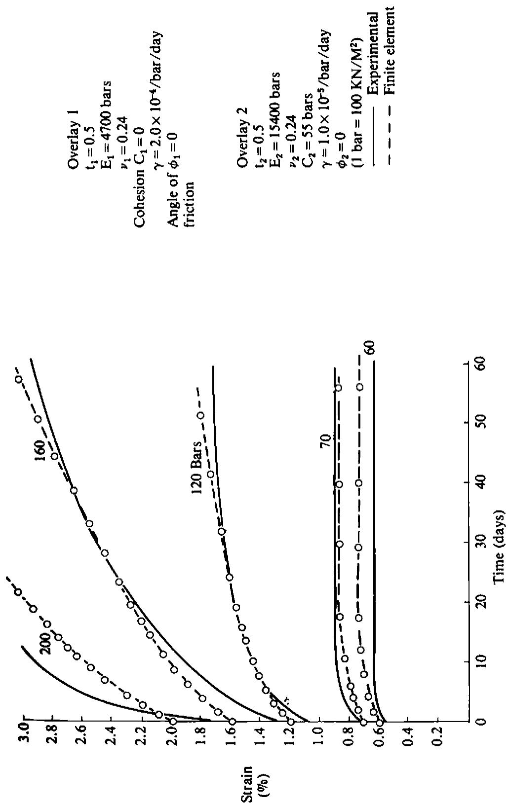
Fig. 8.9 Numerical simulation of experimental creep curves by use of the overlay method.
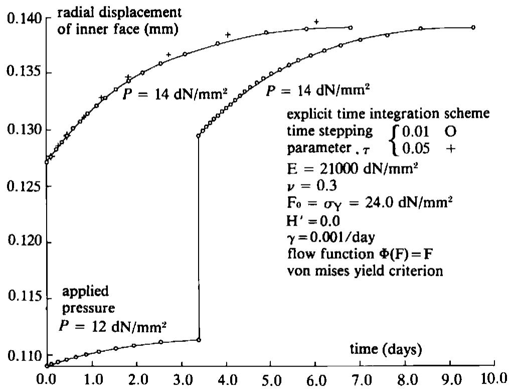
plane strain conditions being assumed in the axial direction. The material properties employed are identical to the case of Fig. 7.12(a) and the fluidity parameter is chosen as $\gamma = 0.001$ . Again a Von Mises yield surface is adopted in solution and the flow function $\Phi(F) = F$ is assumed. An explicit time stepping algorithm ( $\Theta = 0$ ) is initially employed and the radial displacement of the inner surface with time is shown in Fig. 8.10 for two increments of applied pressure. Steady state conditions are allowed to develop for an applied pressure of $12\mathrm{dN/mm}^2$ before a further pressure increment of $2\mathrm{dN/mm}^2$ is added. For each increment the time stepping parameter values $\tau = 0.01$ , $k = 1.5$ were employed, the initial time-step length was chosen as 0.1 days and the steady state convergence tolerance parameter taken as $0.1\%$ . Also shown in Fig. 8.10 are the results for the situation when an internal pressure of $P = 14\mathrm{dN/mm}^2$ is instantaneously applied. The steady state displacement is seen to be in good agreement with that obtained from the two-load
line
| time (days) | radial displacement of inner face (mm) - P = 14 dN/mm² | radial displacement of inner face (mm) - P = 12 dN/mm² |
| ----------- | -------------------------------------------------- | -------------------------------------------------- |
| 0.0 | 0.127 | 0.110 |
| 1.0 | 0.132 | 0.110 |
| 2.0 | 0.135 | 0.110 |
| 3.0 | 0.137 | 0.110 |
| 4.0 | 0.138 | 0.110 |
| 5.0 | 0.139 | 0.110 |
| 6.0 | 0.139 | 0.110 |
| 7.0 | 0.139 | 0.110 |
| 8.0 | 0.139 | 0.110 |
| 9.0 | 0.139 | 0.110 |
| 10.0 | 0.139 | 0.110 |
Fig. 8.10 Displacement of the inner surface with time of an elasto-viscoplastic cylinder subjected to an incrementally applied internal pressure (Mesh of Fig. 7.12(a)).
increment solution. The problem was reanalysed for an applied pressure, $P = 14 \, dN/mm^{2}$ using larger time-step lengths as governed by $\tau = 0.05$ . The loss of accuracy is immediately apparent, with the larger time steps overestimating the viscoplastic strain rates.
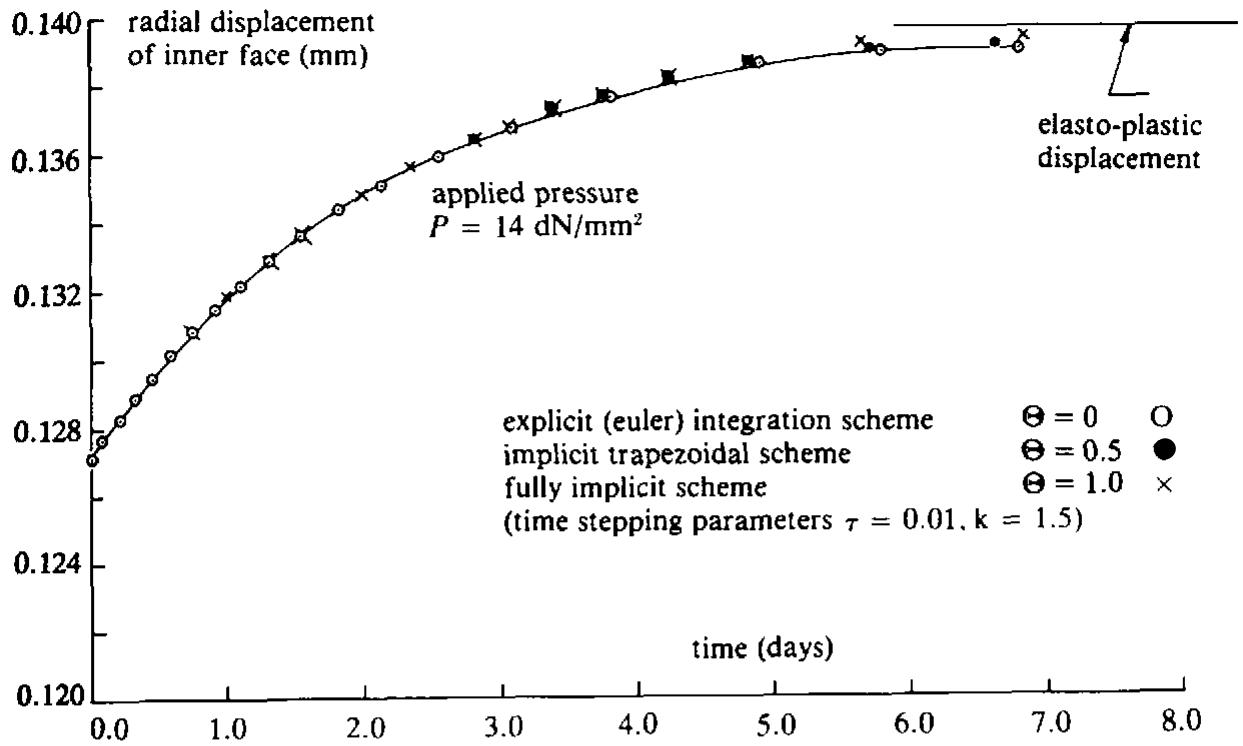
The problem was then resolved using in turn, the implicit trapezoidal time stepping scheme ( $\Theta = \frac{1}{2}$ ) and the full implicit or backward difference scheme ( $\Theta = 1$ ). Good agreement between the three time integration schemes
line
| time (days) | radial displacement of inner face (mm) | scheme |
| ----------- | ------------------------------------- | ------ |
| 0.0 | 0.128 | 0 |
| 0.5 | 0.129 | 0 |
| 1.0 | 0.130 | 0 |
| 1.5 | 0.131 | 0 |
| 2.0 | 0.132 | 0 |
| 2.5 | 0.133 | 0 |
| 3.0 | 0.134 | 0 |
| 3.5 | 0.135 | 0 |
| 4.0 | 0.136 | 0 |
| 4.5 | 0.137 | 0 |
| 5.0 | 0.138 | 0 |
| 5.5 | 0.139 | 0 |
| 6.0 | 0.1395 | 0 |
| 6.5 | 0.1398 | 0 |
| 7.0 | 0.1399 | 0 |
| 7.5 | 0.13995 | 0 |
| 8.0 | 0.13998 | 0 |
| 0.0 | 0.128 | 0.5 |
| 0.5 | 0.129 | 0.5 |
| 1.0 | 0.130 | 0.5 |
| 1.5 | 0.131 | 0.5 |
| 2.0 | 0.132 | 0.5 |
| 2.5 | 0.133 | 0.5 |
| 3.0 | 0.134 | 0.5 |
| 3.5 | 0.135 | 0.5 |
| 4.0 | 0.136 | 0.5 |
| 4.5 | 0.137 | 0.5 |
| 5.0 | 0.138 | 0.5 |
| 5.5 | 0.139 | 0.5 |
| 6.0 | 0.1395 | 0.5 |
| 6.5 | 0.1398 | 0.5 |
| 7.0 | 0.1399 | 0.5 |
| 7.5 | 0.13995 | 0.5 |
| 8.0 | 0.13998 | 0.5 |
| 0.0 | 0.128 | 1.0 |
| 0.5 | 0.129 | 1.0 |
| 1.0 | 0.130 | 1.0 |
| 1.5 | 0.131 | 1.0 |
| 2.0 | 0.132 | 1.0 |
| 2.5 | 0.133 | 1.0 |
| 3.0 | 0.134 | 1.0 |
| 3.5 | 0.135 | 1.0 |
| 4.0 | 0.136 | 1.0 |
| 4.5 | 0.137 | 1.0 |
| 5.0 | 0.138 | 1.0 |
| 5.5 | 0.139 | 1.0 |
| 6.0 | 0.1395 | 1.0 |
| 6.5 | 0.1398 | 1.0 |
| 7.0 | 0.1399 | 1.0 |
| 7.5 | 0.13995 | 1.0 |
| 8.0 | 0.13998 | 1.0 |
| 0.0 | 0.128 | 0 |
| 0.5 | 0.129 | 0 |
| 1.0 | 0.130 | 0 |
| 1.5 | 0.131 | 0 |
| 2.0 | 0.132 | 0 |
| 2..5 | 0.133 | 0 |
| 3.0 | 0.134 | 0 |
| 3.5 | 0.135 | 0 |
| 4.0 | 0.136 | 0 |
| 4.5 | 0.137 | 0 |
| 5.0 | 0.0000 | 0 |
| 5.5 | 0.0000 | 0 |
| 6.0 | 0.0000 | 0 |
| 6.5 | 0.0000 | 0 |
| 7.0 | 0.0000 | 0 |
| 7.5 | 0.0000 | 0 |
| 8.0 | 0.0000 | 0 |
Fig. 8.11 Comparison of various time integration schemes for the internally pressurised cylinder of Fig. 8.10.
line
| Applied Pressure (mm) | Elastic Solution (dN/mm²) | Elastoplastic Solution (dN/mm²) |
| --------------------- | ------------------------ | ------------------------------- |
| 100 | 22.0 | 14.5 |
| 200 | 18.0 | 17.0 |
| 300 | 16.0 | 15.0 |
| 400 | 14.0 | 13.0 |
| 500 | 12.0 | 11.0 |
| 600 | 10.0 | 9.0 |
| 700 | 8.0 | 7.0 |
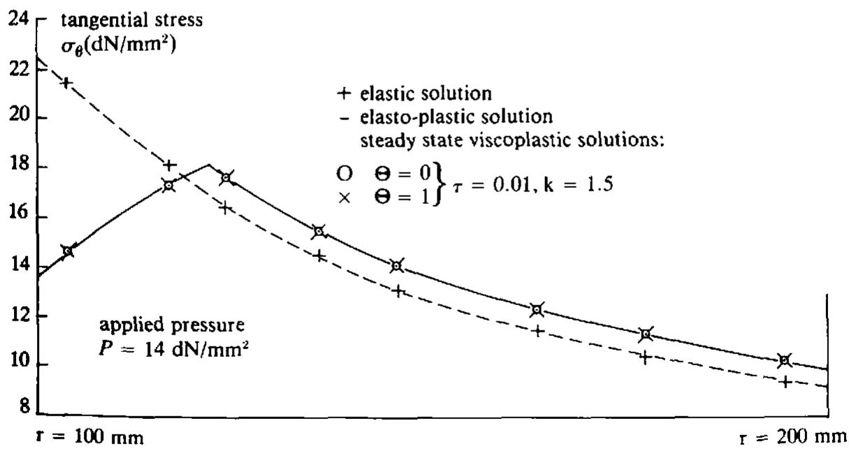
Fig. 8.12 Steady state tangential stress distribution in an elasto-viscoplastic internally pressurised cylinder.
is evident in Fig. 8.11 with the steady state displacement in each case comparing well with the corresponding elasto-plastic value of Fig. 7.12(b).
The steady state hoop stress distributions are shown in Fig. 8.12 for the time integration schemes $\Theta = 0$ and $\Theta = 1$ , and the results are compared with the elasto-plastic solution of Fig. 7.13. Excellent agreement is obtained
as required; since theoretically the steady state viscoplastic solution coincides with the corresponding elasto-plastic solution.
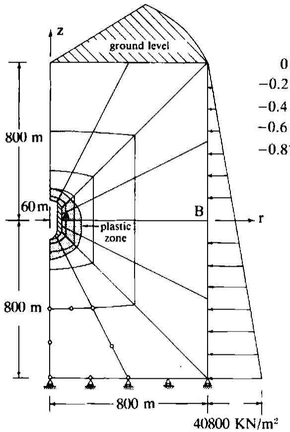
The problem of the stresses induced in the vicinity of an excavated underground storage cavity is illustrated in Fig. 8.13. Applications in this area include oil and gas reservoirs, nuclear waste disposal and geothermal energy problems. The cavity is assumed to be axisymmetric and Fig. 8.13
text_image
ground level
z
0
-0.2
-0.4
-0.6
-0.8
800 m
60 m
plastic
zone
B
r
800 m
800 m
40800 KN/m²
line
| Point | Value (m) |
|-------|-----------|
| A | 0.0 |
| B | -0.6 |
gravity and pressure loading
instantaneously applied at time, t = 0
$$
\mathrm{E} = 6. 9 \times 1 0 ^ {5} \mathrm{KN} / \mathrm{m} ^ {2}
$$
$$
\nu = 0. 4
$$
$$
\rho = 2 5 5 0 \mathrm{Kg} / \mathrm{m} ^ {3}
$$
$$
\mathrm{F} _ {0} = 1 0 0 0 0 \mathrm{KN} / \mathrm{m} ^ {2}
$$
$$
\gamma = 0. 0 7 5 / \text { y e a r }
$$
$$
\Phi (\mathbf {F}) = \mathbf {F}
$$
$$
\mathbf {H} ^ {\prime} = 0. 0
$$
Von mises yield criterion
explicit time integration, $\tau = 0.05$
steady state conditions
achieved in 0.7 years.
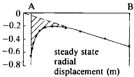
Fig. 8.13 Elasto-viscoplastic analysis of a subterranean cavity, showing zones of plasticity and steady state radial displacement at mid-height.
shows the finite element idealisation of a cylindrical portion of the surrounding rock mass. Before excavation of the cavity the tectonic stress field in the rock is assumed to be hydrostatic. This condition is simulated by a gravity loading together with a lateral hydrostatic pressure applied to the cylindrical face of the model. The material properties employed are indicated in Fig. 8.13. The cavity is assumed to be instantaneously excavated at time t = 0 and viscoplastic solution to steady state conditions performed by explicit time integration ( $\Theta = 0$ ). Steady state conditions are achieved in 0.7 years and the zones of viscoplastic deformation at this time are illustrated in Fig. 8.13. It should be emphasised that since the fluidity parameter $\gamma$ only enters the viscoplastic expressions through the product $\gamma.t$ , then solution for different material fluidity values simply necessitates an adjustment of the time scale. Figure 8.13 also shows the radial displacement along section AB at steady state. The displacement distribution is seen to be made up of a
line
| radial stress, σr (KN/m²) | Value |
| ------------------------- | --------- |
| 0 | 0 |
| 1000 | -2000 |
| 2000 | -4000 |
| 3000 | -6000 |
| 4000 | -8000 |
| 5000 | -10000 |
| 6000 | -12000 |
| 7000 | -14000 |
| 8000 | -16000 |
| 9000 | -18000 |
| 10000 | -20000 |
| 11000 | -21000 |
| 12000 | -22000 |
| 13000 | -22500 |
| 14000 | -22500 |
| 15000 | -22500 |
line
| tangential stress. σ_H (KN/m²) | Value |
| ----------------------------- | --------- |
| -1000 | 0 |
| -800 | -10000 |
| -600 | -12000 |
| -400 | -15000 |
| -200 | -18000 |
| 0 | -23000 |
| 200 | -23000 |
| 400 | -23000 |
| 600 | -23000 |
| 800 | -23000 |
| 1000 | -23000 |
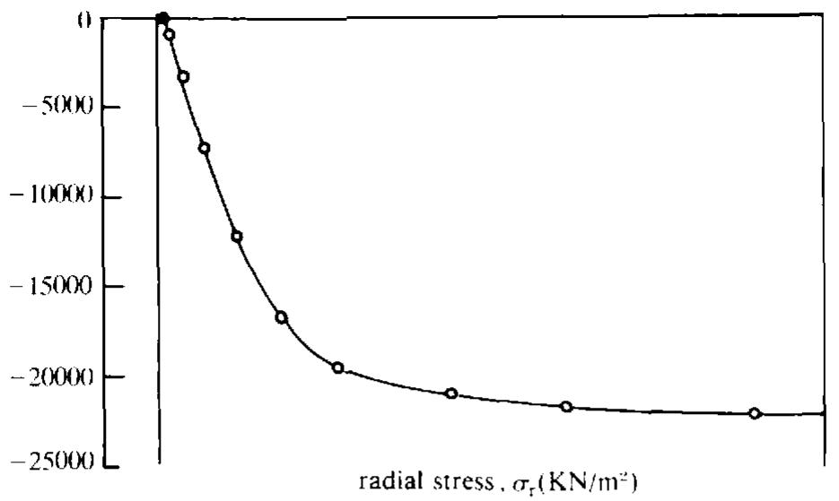
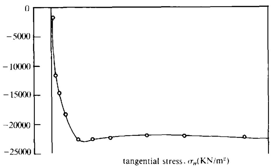
Fig. 8.14 Radial and tangential stress distributions for the problem of Fig. 8.13.
linear field caused by the external applied pressure, superimposed on which is the effect of the cavity presence (the shaded area).
Finally, Fig. 8.14 shows the steady state radial and tangential stress distributions along the line of Gaussian integration points nearest section AB. It is noted that away from the vicinity of the cavity, the hydrostatic condition $\sigma_{r} = \sigma_{0}$ is reproduced.
# 8.17 Problems
8.1 Use program VISCOUNT documented in Appendix II, Section A2.2 to solve the thick sphere considered in Problem 7.5 for the viscoplastic case. Employ the same material properties and load increment sizes as used in the elasto-plastic analysis. Assume the fluidity parameter
$\gamma = 0.001$ and flow function $\Phi(F) = F$ . Use explicit time integration $(\Theta = 0)$ and compare your steady state solutions with the results of Problem 7.5.
8.2 Repeat Problem 8.1 for different limiting time step lengths employing explicit time integration. Take the factor $\tau$ , described in Section 8.3, in the range $0.01 \leqslant \tau \leqslant 0.5$ . Comment on the accuracy of solution in each case.
8.3 Repeat Problem 8.1 using the flow functions (8.8) and (8.9). Take the indices M and N in the range 2 to 4. Comment on the solutions.
8.4 Repeat Problem 8.1 using (a) Fully implicit method ( $\Theta = 1$ ) and (b) Implicit trapezoidal rule ( $\Theta = \frac{1}{2}$ ). Comment on the accuracy and computational costs of solution.
8.5 Modify program VISCOUNT to include the strain-hardening law considered in Problem 7.4.
8.6 Undertake all the coding changes required to program VISCOUNT to include the overlay concept described in Section 8.15.
8.7 Test the modified program of Problem 8.6 by employing it in the solution of the uniaxial problem of Fig. 8.15. A constant stress of 100 is applied at time t = 0 to the plane stress model shown. Determine the development of strain with time. Verify the numerical solution by noting Figs. 8.4 and 8.5 and hence comparing with the analytical solution of Problem 4.2.
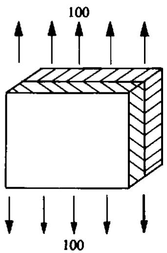
text_image
100
100
| Overlay 1 | Overlay 2 |
| E | 1000.0 | 1000.0 |
| $\nu$ | 0.0 | 0.0 |
| t | 0.5 | 0.5 |
| $\sigma_{\gamma}$ | 0.0 | 25.0 |
| H' | 100.0 | 100.0 |
| $\gamma$ | 0.01 | 0.01 |
Fig. 8.15 Overlay model example—Problem 8.7.
8.8 In Section 8.2.3 it was stated that large deformation effects could be included, adopting a Lagrangian formulation, by including both the linear and nonlinear terms of the general quadratic relationship between strains and displacements according to (8.19). Details of geometrically nonlinear expressions can be found in Chapters 10 and 11. Modify program VISCOUNT to include such geometrically nonlinear behaviour.
8.9 Employ the modified program of Problem 8.8 to solve the creep buckling problem illustrated in Fig. 8.16. The creep law employed is indicated in Fig. 8.16 and is a particular form of expression (8.9). Using the finite element mesh shown, apply the eccentric load to the cantilever at time, t = 0, and employ the implicit time integration algorithm ( $\Theta = 1$ ) to determine the deformation with increasing time. At some stage of the solution process the structure will become unstable due to creep buckling. Carry out the analysis for $\lambda = 1.0, 1.5, 2.0$ and 2.5 and compare the lateral deflection/time relationships with those provided in Ref. 6.
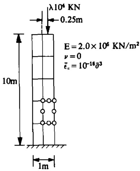
text_image
λ10⁴ KN
0.25m
E = 2.0 × 10⁶ KN/m²
ν = 0
ε̅c = 10⁻¹⁶σ̅³
10m
1m
Fig. 8.16 Creep buckling example—Problem 8.9.
8.10 Modify program VISCOUNT to undertake the elasto-viscoplastic solution of three-dimensional solids. The majority of the subroutines required have been already modified in Problem 7.9.
8.11 Repeat Problem 7.10 for the elasto-viscoplastic program VISCOUNT.
# 8.18 References
1. OLSZAK, W. and PERZYNA, P., Stationary and non-stationary visco-plasticity, In: M. F. Kanninen et al. (Eds), Inelastic Behaviour of Solids, McGraw-Hill, 1970.
2. OLSZAK, W. and PERZYNA, P., On elasto-viscoplastic soils, In: Rheology and Soil Mechanics, IUTAM Symposium, Springer-Verlag, Grenoble, 1966.
3. PERZYNA, P., Fundamental problems in visco-plasticity, In: Recent Advances in Applied Mechanics, Academic Press, New York, 1966.
4. ZIENKIEWICZ, O. C. and CORMEAU, I. C., Visco-plasticity—plasticity and creep in elastic solids—a unified numerical solution approach, Int. J. Num. Meth. Engng. 8, 821–845 (1974).
5. ZIENKIEWICZ, O. C., OWEN, D. R. J. and CORMEAU, I. C., Analysis of viscoplastic effects in pressure vessels by the finite element method, Nuclear Engineering & Design, 28(2), 278–288 (1974).
§. KANCHI, M. B., ZIENKIEWICZ, O. C. and OWEN, D. R. J., The visco-plastic approach to problems of elasticity and creep involving geometric nonlinear effects. Int. J. Num. Meth. Engng. 12, 169–181 (1978).
7. STRICKLIN, J. A., HAISLER, W. and REISEMANN, W., Evaluation of solution procedures of material and/or geometrically non-linear structural analysis, AIAA J. 11, 292–299 (1973).
8. DINIS, L. M. S. and OWEN, D. R. J., Elastic-viscoplastic analysis of plates by the finite element method, Computers & Structures, 8, 207-215 (1978).
9. CORMEAU, I., Numerical stability in quasistatic elasto-visco-plasticity, Int. J. Num. Meth. Engng. 9, 109–127 (1975).
10. Duwez, P., On the Plasticity of Crystals, Physical Review, 47(6), 494–501 (1935).
11. ZIENKIEWICZ, O. C., NAYAK, G. C. and OWEN, D. R. J., Composite and overlay models in numerical analysis of elasto-plastic continua, Int. Symp. Foundations of Plasticity, Warsaw (1972).
12. OWEN, D. R. J., PRAKASH, A. and ZIENKIEWICZ, O. C., Finite element analysis of non-linear composite materials by use of overlay systems, Computers & Structures 4, 1251–1267 (1974).
13. PANDE, G. N., OWEN, D. R. J and ZIENKIEWICZ, O. C., Overlay models in time-dependent nonlinear material analysis. Computers & Structures, 7, 435-443 (1977).
14. HUGHES, T. J. R. and TAYLOR, R. L., Unconditionally stable algorithms for quasi-static elasto/viscoplastic finite element analysis, Int. J. Num. Meth. Engng. (to be published).
# Chapter 9 Elasto-plastic Mindlin plate bending analysis
Written in collaboration with M. M. Huq
# 9.1 Introduction
In Chapter 5 we introduced some elastoplastic Timoshenko beam formulations. In this chapter we introduce some related elasto-plastic Mindlin plate bending formulations.
There are basically three theories which we could use as a basis for elastic plate bending:
(i) Kirchhoff classical thin plate theory This theory, which takes no account of transverse shear deformation, is usually favoured by engineers because of its simplicity. It is the plate bending equivalent of Euler–Bernoulli beam theory. Many conforming $C(1)$ and non-conforming $C(0)$ plate elements are available.
(ii) Mindlin (or Reissner) plate theory. Mindlin and the related Reissner plate theories allow for transverse shear effects. Mindlin plate theory is the plate bending equivalent of Timoshenko beam theory. Several Mindlin plate elements have been presented in the literature and it emerges that the most convenient one is the 'Heterosis' element of Hughes. $^{(1)}$
(iii) Full three-dimensional theory. For the greatest accuracy, full three-dimensional theory should be employed. Many 3D hexahedral and tetrahedral elements have been presented. Unfortunately when the aspect ratio of the element is very large as in thin plates, an ill-conditioned stiffness matrix results and roundoff problems predominate. Several schemes for avoiding this difficulty have been presented and undoubtedly an analysis based on this procedure is the most accurate.
Let us now consider the various possibilities for elasto-plastic analysis.
(i) We could use a full 3D analysis with a yield function $F(\sigma_x, \sigma_y, \sigma_z, \tau_{xy}, \tau_{xz}, \tau_{yz})$ .
(ii) In a Mindlin plate formulation we can also use the yield function $F(\sigma_x, \sigma_y, \sigma_z, \tau_{xy}, \tau_{xz}, \tau_{yz})$ . It should be noted that $\sigma_z$ is taken as zero in
Mindlin plates. This approach allows for the spread of plasticity from the extreme fibre over the entire plate thickness. In the evaluation of the internal virtual work integrals we may sample the stresses of the Gauss-Legendre or Lobatto integration points. Alternatively we may divide the plate into layers and use a mid-ordinate rule.
(iii) In a Mindlin or Kirchhoff formulation we can use a yield function $F(\sigma_x, \sigma_y, \tau_{xy})$ . In Mindlin plate theory we ignore the effect of $\tau_{xz}$ and $\tau_{yz}$ on the plastic behaviour. Since, in the absence of inplane forces, the inplane stresses are a maximum at the extreme fibres where the transverse shear stresses are a minimum and the inplane stresses are a minimum at the mid-plane where the transverse shears are a maximum, this is a reasonable assumption. (There is also further evidence to suggest that it is likely to lead to insignificant errors.) This approach also allows for the spread of plasticity over the depth of the plate. In the evaluation of the internal virtual work integrals we may sample the stresses at the Gauss–Legendre or Lobatto integration points. Alternatively we may divide the plate into layers\* and use a mid-ordinate rule. This ‘layered’ approach has been described in Chapter 5 for a Timoshenko beam element and is a very popular method.
(iv) In a Mindlin or Kirchhoff formulation we can adopt in the absence of inplane forces a yield function $F(M_x, M_y, M_{xy})$ which is a function of the bending moments. Here it is assumed that at a point the whole plate section becomes plastic simultaneously. A similar approach was described in Chapter 5 for Timoshenko beam elements.
The elasto-plastic analysis of Mindlin plates is considered in this chapter, where both layered and non-layered approaches are treated in detail.
Finite elements based on Mindlin's assumptions have one important advantage over elements based on classical thin plate theory. Mindlin plate elements require only $C(0)$ continuity of the lateral displacement $w$ and the two independent nodal rotations $\theta_x$ and $\theta_y$ . However elements based on classical Kirchhoff thin plate theory require $C(1)$ continuity; in other words $\partial w / \partial x$ and $\partial w / \partial y$ as well as $w$ must be continuous across element interfaces. Thus, Mindlin plate elements are simpler to formulate and they have the added advantage of being able to model shear-weak as well as shear-stiff plates. Consequently, if transverse shear deformations are present they are automatically modelled with Mindlin elements.
Recent research $^{(1)}$ indicates that the use of a ‘Heterosis’ quadrilateral Mindlin plate element with quadratic Lagrangian interpolation for $\theta_{x}$ and $\theta_{y}$ and quadratic Serendipity interpolation for w together with selective integration of the stiffness matrix, gives the best overall performance. It