Evaluate the components of the force in the primed coordinate system in Fig. E2.24. Here we have, using (2.56), $$ \mathbf {P} = \left[ \begin{array}{c c c} 1 & 0 & 0 \\ 0 & \cos \theta & \sin \theta \\ 0 & - \sin \theta & \cos \theta \end{array} \right] $$ and then $$ \mathbf {R} ^ {\prime} = \mathbf {P R} \tag {a} $$ where $\mathbf{R}'$ gives the components of the force in the primed coordinate system. As a check, if we use $\theta = -30^{\circ}$ we obtain, using (a), $$ \mathbf {R} ^ {\prime} = \left[ \begin{array}{l} 0 \\ 0 \\ 2 \end{array} \right] $$ which is correct because the $e_{3}^{\prime}$ -vector is now aligned with the force vector. To define a second-order tensor we build on the definition given in (2.54) for a tensor of rank 1. Definition: An entity is called a second-order tensor if it has nine components $t_{ij}$ , $i = 1, 2, 3$ , and $j = 1, 2, 3$ , in the unprimed frame and nine components $t_{ij}'$ in the primed frame and if these components are related by the characteristic law $$ t _ {i j} ^ {\prime} = p _ {i k} p _ {j l} t _ {k l} \tag {2.60} $$ As in the case of the definition of a first-order tensor, the relation in $(2.60)$ represents a change of basis in the representation of the entity (see Example 2.25) and we can formally derive $(2.60)$ in essentially the same way as we derived $(2.54)$ . That is, if we write the same tensor of rank 2 in the two different bases, we obtain $$ t _ {m n} ^ {\prime} \mathbf {e} _ {m} ^ {\prime} \mathbf {e} _ {n} ^ {\prime} = t _ {k l} \mathbf {e} _ {k} \mathbf {e} _ {l} \tag {2.61} $$ where clearly in the tensor representation the first base vector goes with the first subscript (the row in the matrix representation) and the second base vector goes with the second subscript (the column in the matrix representation). The open product $^{1}$ or tensor product $e_{k}e_{l}$ is called a dyad and a linear combination of dyads as used in (2.61) is called a dyadic, (see, for example, L. E. Malvern [A]). Taking the dot product from the right in (2.61), first with $\mathbf{e}_j'$ and then with $\mathbf{e}_i'$ , we obtain $$ t _ {m n} ^ {\prime} \mathbf {e} _ {m} ^ {\prime} \delta_ {n j} = t _ {k l} \mathbf {e} _ {k} \left(\mathbf {e} _ {l} \cdot \mathbf {e} _ {j} ^ {\prime}\right) $$ $$ t _ {m n} ^ {\prime} \delta_ {m i} \delta_ {n j} = t _ {k l} \left(\mathbf {e} _ {k} \cdot \mathbf {e} _ {i} ^ {\prime}\right) \left(\mathbf {e} _ {l} \cdot \mathbf {e} _ {j} ^ {\prime}\right) \tag {2.62} $$ or $$ t _ {i j} ^ {\prime} = t _ {k l} p _ {i k} p _ {j l} $$ $^{1}$ The open product or tensor product of two vectors denoted as ab is defined by the requirement that $$ (\mathbf {a b}) \cdot \mathbf {v} = \mathbf {a} (\mathbf {b} \cdot \mathbf {v}) $$ for all vectors v. Some writers use the notation a ⊗ b instead of ab. Here $\delta_{ij}$ is the Kronecker delta ( $\delta_{ij} = 1$ for $i = j$ , and $\delta_{ij} = 0$ for $i \neq j$ ). This transformation may also be written in matrix form as $$ \mathbf {t} ^ {\prime} = \mathbf {P} \mathbf {t} \mathbf {P} ^ {T} \tag {2.63} $$ where the $(i, k)$ th element in $\mathbf{P}$ is given by $p_{ik}$ . Of course, the inverse transformation also holds: $$ \mathbf {t} = \mathbf {P} ^ {T} \mathbf {t} ^ {\prime} \mathbf {P} \tag {2.64} $$ This relation can be derived using (2.61) and [similar to the operation in (2.62)] taking the dot product from the right with $e_{j}$ and then $e_{i}$ , or simply using (2.63) and the fact that P is an orthogonal matrix. In the preceding definitions we assumed that all indices vary from 1 to 3; special cases are when the indices vary from 1 to n, with n < 3. In engineering analysis we frequently deal only with two-dimensional conditions, in which case n = 2. 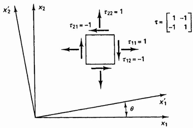EXAMPLE 2.25: Stress is a tensor of rank 2. Assume that the stress at a point measured in an unprimed coordinate frame in a plane stress analysis is (not including the third row and column of zeros) $$ \boldsymbol {\tau} = \left[ \begin{array}{c c} 1 & - 1 \\ - 1 & 1 \end{array} \right] $$ Establish the components of the tensor in the primed coordinate system shown in Fig. E2.25. 

text_image

x₂' x₂ τ₂₁ = -1 τ₂₂ = 1 τ₁₁ = 1 τ₁₂ = -1 τ = [1 -1] -1 1] θ x₁' x₁

Figure E2.25 Representation of a stress tensor in different coordinate systems Here we use the rotation matrix $\mathbf{P}$ as in Example 2.24, and the transformation in (2.63) is $$ \boldsymbol {\tau} ^ {\prime} = \mathbf {P} \boldsymbol {\tau} \mathbf {P} ^ {T}; \quad \mathbf {P} = \left[ \begin{array}{c c} \cos \theta & \sin \theta \\ - \sin \theta & \cos \theta \end{array} \right] $$ Assume that we are interested in the specific case when $\theta = 45^{\circ}$ . In this case we have $$ \boldsymbol {\tau} ^ {\prime} = \frac {1}{2} \left[ \begin{array}{l l} 1 & 1 \\ - 1 & 1 \end{array} \right] \left[ \begin{array}{l l} 1 & - 1 \\ - 1 & 1 \end{array} \right] \left[ \begin{array}{l l} 1 & - 1 \\ 1 & 1 \end{array} \right] = \left[ \begin{array}{l l} 0 & 0 \\ 0 & 2 \end{array} \right] $$ and we recognize that in this coordinate system the off-diagonal elements of the tensor (shear components) are zero. The primed axes are called the principal coordinate axes, and the diagonal elements $\tau_{11}^{\prime}=0$ and $\tau_{22}^{\prime}=2$ are the principal values of the tensor. We will see in Section 2.5 that the principal tensor values are the eigenvalues of the tensor and that the primed axes define the corresponding eigenvectors. The previous discussion can be directly expanded to also define tensors of higher order than 2. In engineering analysis we are, in particular, interested in the constitutive tensors that relate the components of a stress tensor to the components of a strain tensor (see, for example, Sections 4.2.3 and 6.6) $$ \tau_ {i j} = C _ {i j k l} \epsilon_ {k l} \tag {2.65} $$ The stress and strain tensors are both of rank 2, and the constitutive tensor with components $C_{ijkl}$ is of rank 4 because its components transform in the following way: $$ C _ {i j k l} ^ {\prime} = p _ {i m} p _ {j n} p _ {k r} p _ {l s} C _ {m n r s} \tag {2.66} $$ In the above discussion we used the orthogonal base vectors $e_{i}$ and $e_{j}^{\prime}$ of two Cartesian systems. However, we can also express the tensor in components of a basis of nonorthogonal base vectors. It is particularly important in shell analysis to be able to use such base vectors (see Sections 5.4.2 and 6.5.2). 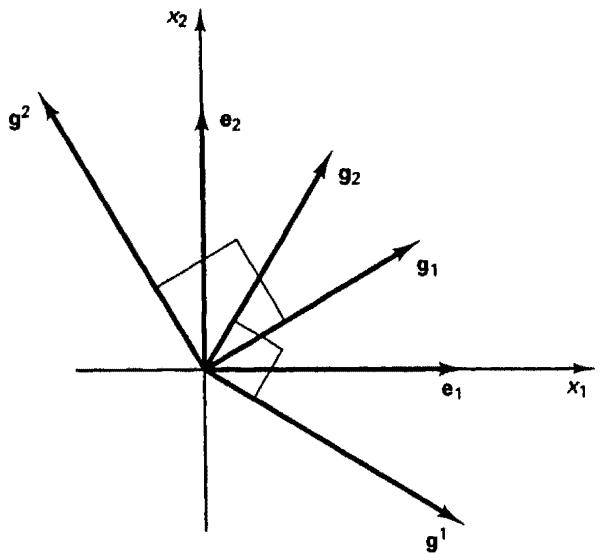In continuum mechanics it is common practice to use what is called a covariant basis with the covariant base vectors $g_{i}, i = 1, 2, 3$ , and what is called a contravariant basis with the contravariant base vectors, $g^{j}, j = 1, 2, 3$ ; see Fig. 2.5 for an example. The covariant and contravariant base vectors are in general not of unit length and satisfy the relationships $$ \mathbf {g} _ {i} \cdot \mathbf {g} ^ {j} = \delta_ {i} ^ {j} \tag {2.67} $$ where $\delta_{i}^{j}$ is the (mixed) Kronecker delta ( $\delta_{i}^{j} = 1$ for $i = j$ , and $\delta_{i}^{j} = 0$ for $i \neq j$ ). 

text_image

x₂ g² e₂ g₂ g₁ e₁ x₁ g¹

$$ \mathbf {g} _ {1} \cdot \mathbf {g} ^ {1} = 1; \quad \mathbf {g} _ {2} \cdot \mathbf {g} ^ {1} = 0 $$ $$ \mathbf {g} _ {1} \cdot \mathbf {g} ^ {2} = 0; \quad \mathbf {g} _ {2} \cdot \mathbf {g} ^ {2} = 1 $$ Figure 2.5 Example of covariant and contravariant base vectors, n = 2 (plotted in Cartesian reference frame) Hence the contravariant base vectors are orthogonal to the covariant base vectors. Furthermore, we have $$ \mathbf {g} _ {i} = g _ {i j} \mathbf {g} ^ {j} \tag {2.68} $$ with $g_{ij} = \mathbf{g}_i\cdot \mathbf{g}_j$ (2.69) and $\mathbf{g}^i = g^{ij}\mathbf{g}_j$ (2.70) with $g^{ij} = \mathbf{g}^i\cdot \mathbf{g}^j$ (2.71) where $g_{ij}$ and $g^{ij}$ are, respectively, the covariant and contravariant components of the metric tensor. To prove that (2.68) holds, we tentatively let $$ \mathbf {g} _ {i} = a _ {i k} \mathbf {g} ^ {k} \tag {2.72} $$ with the $a_{ik}$ unknown elements. Taking the dot product on both sides with $g_{j}$ , we obtain $$ \begin{array}{l} \mathbf {g} _ {i} \cdot \mathbf {g} _ {j} = a _ {i k} \mathbf {g} ^ {k} \cdot \mathbf {g} _ {j} \\ = a _ {i k} \delta_ {j} ^ {k} \tag {2.73} \\ = a _ {i j} \\ \end{array} $$ Of course, (2.70) can be proven in a similar way (see Exercise 2.11). Frequently, in practice, the covariant basis is conveniently selected and then the contravariant basis is given by the above relationships. 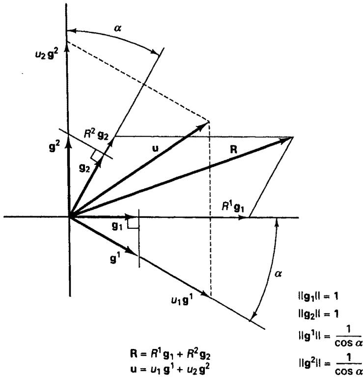Assume that we need to use a basis with nonorthogonal base vectors. The elegance of then using both the covariant and contravariant base vectors is seen if we simply consider the work done by a force R going through a displacement u, given by $R \cdot u$ . If we express both R and u in the covariant basis given by the base vectors $g_{i}$ , we have $$ \begin{array}{l} \mathbf {R} \cdot \mathbf {u} = \left(R ^ {1} \mathbf {g} _ {1} + R ^ {2} \mathbf {g} _ {2} + R ^ {3} \mathbf {g} _ {3}\right) \cdot \left(u ^ {1} \mathbf {g} _ {1} + u ^ {2} \mathbf {g} _ {2} + u ^ {3} \mathbf {g} _ {3}\right) \\ = R ^ {i} u ^ {j} g _ {i j} \tag {2.74} \\ \end{array} $$ On the other hand, if we express only $\mathbf{R}$ in the covariant basis, but $\mathbf{u}$ in the contravariant basis, given by the base vectors $\mathbf{g}^j$ , we have $$ \begin{array}{l} \mathbf {R} \cdot \mathbf {u} = \left(R ^ {1} \mathbf {g} _ {1} + R ^ {2} \mathbf {g} _ {2} + R ^ {3} \mathbf {g} _ {3}\right) \cdot \left(u _ {1} \mathbf {g} ^ {1} + u _ {2} \mathbf {g} ^ {2} + u _ {3} \mathbf {g} ^ {3}\right) = R ^ {i} u _ {j} \delta_ {i} ^ {j} \\ = R ^ {i} u _ {i} \tag {2.75} \\ \end{array} $$ which is a much simpler expression. Fig. 2.6 gives a geometrical representation of this evaluation in a two-dimensional case. We shall use covariant and contravariant bases in the formulation of plate and shell elements. Since we are concerned with the product of stress and strain (e.g., in the principle of virtual work), we express the stress tensor in contravariant components [as for the force $\mathbf{R}$ in (2.75)], $$ \tau = \tilde {\tau} ^ {m n} \mathbf {g} _ {m} \mathbf {g} _ {n} \tag {2.76} $$ and the strain tensor in covariant components [as for the displacement in (2.75)], $$ \epsilon = \tilde {\epsilon} _ {i j} \mathbf {g} ^ {i} \mathbf {g} ^ {j} \tag {2.77} $$ 

text_image

u₂g² α R²g₂ g² u R R¹g₁ g₁ g¹ u₁g¹ α ||g₁|| = 1 ||g₂|| = 1 ||g¹|| = 1/cos α ||g²|| = 1/cos α R = R¹g₁ + R²g₂ u = u₁g¹ + u₂g²

Figure 2.6 Geometrical representation of R and u using covariant and contravariant bases Using these dyadics we obtain for the product of stress and strain $$ \begin{array}{l} W = \left(\tilde {\tau} ^ {m n} \mathbf {g} _ {m} \mathbf {g} _ {n}\right) \cdot \left(\tilde {\epsilon} _ {i j} \mathbf {g} ^ {i} \mathbf {g} ^ {j}\right) \\ = \tilde {\tau} ^ {m n} \tilde {\epsilon} _ {i j} \delta_ {m} ^ {i} \delta_ {n} ^ {j} \tag {2.78} \\ = \tilde {\tau} ^ {i j} \tilde {\epsilon} _ {i j} \\ \end{array} $$ This expression for W is as simple as the result in (2.75). Note that here we used the convention—designed such that its use leads to correct results $^{2}$ —that in the evaluation of the dot product the first base vector of the first tensor multiplies the first base vector of the second tensor, and so on. Instead of writing the product in summation form of products of components, we shall also simply use the notation $$ W = \tau \cdot \epsilon \tag {2.79} $$ and simply imply the result in (2.78), in whichever coordinate system it may be obtained. The notation in (2.79) is, in essence, a simple extension of the notation of a dot product between two vectors. Of course, when considering $u \cdot v$ , a unique result is implied, but this result can be obtained in different ways, as given in (2.74) and (2.75). Similarly, when $^{2}$ Namely, consider (ab) · (cd). Let A = ab, B = cd; then A · B = $A_{ij}B_{ij} = a_{i}b_{j}c_{i}d_{j} = (a_{i}c_{i})(b_{j}d_{j}) = (a \cdot c)(b \cdot d)$ . writing (2.79), the unique result of W is implied, and this result may also be obtained in different ways, but the use of $\tilde{\tau}^{ij}$ and $\tilde{\epsilon}_{ij}$ can be effective (see Example 2.26). Hence we note that the covariant and contravariant bases are used in the same way as Cartesian bases but provide much more generality in the representation and use of tensors. Consider the following examples. EXAMPLE 2.26: Assume that the stress and strain tensor components at a point in a continuum corresponding to a Cartesian basis are $\tau_{ij}$ and $\epsilon_{ij}$ and that the strain energy, per unit volume, is given by $U = \frac{1}{2}\tau_{ij}\epsilon_{ij}$ . Assume also that a basis of covariant base vectors $\mathbf{g}_i$ , $i = 1, 2, 3$ , is given. Show explicitly that the value of $U$ is then also given by $\frac{1}{2}\tilde{\tau}^{mn}\tilde{\epsilon}_{mn}$ . Here we use $$ \tilde {\tau} ^ {m n} \mathbf {g} _ {m} \mathbf {g} _ {n} = \tau_ {i j} \mathbf {e} _ {i} \mathbf {e} _ {j} \tag {a} $$ and $\tilde{\epsilon}_{mn}\mathbf{g}^{m}\mathbf{g}^{n} = \epsilon_{ij}\mathbf{e}_{i}\mathbf{e}_{j}$ (b) But from (a) and (b) we obtain $$ \tau_ {k l} = \tilde {\tau} ^ {m n} (\mathbf {g} _ {m} \cdot \mathbf {e} _ {k}) (\mathbf {g} _ {n} \cdot \mathbf {e} _ {l}) \quad \text { sum on } m \text { and } n $$ and $\epsilon_{kl} = \tilde{\epsilon}_{mn}(\mathbf{g}^m\cdot \mathbf{e}_k)(\mathbf{g}^n\cdot \mathbf{e}_l)$ sum on $m$ and $n$ Now since $$ (\mathbf {g} _ {i} \cdot \mathbf {e} _ {j}) (\mathbf {g} ^ {i} \cdot \mathbf {e} _ {j}) = 1 \quad \text { sum on } j $$ we also have $U = \frac{1}{2}\bar{\tau}^{mn}\tilde{\epsilon}_{mn}$ EXAMPLE 2.27: The Cartesian components $\tau_{ij}$ of the stress tensor $\tau_{ij}e_{i}e_{j}$ are $\tau_{11}=100$ , $\tau_{12}=60$ , $\tau_{22}=200$ , and the components $\epsilon_{ij}$ of the strain tensor $\epsilon_{ij}e_{i}e_{j}$ are $\epsilon_{11}=0.001$ , $\epsilon_{12}=0.002$ , $\epsilon_{22}=0.003$ . Assume that the stress and strain tensors are to be expressed in terms of covariant strain components and contravariant stress components with $$ \mathbf {g} _ {1} = \left[ \begin{array}{l} 1 \\ 0 \end{array} \right]; \quad \mathbf {g} _ {2} = \left[ \begin{array}{l} \frac {1}{\sqrt {2}} \\ \frac {1}{\sqrt {2}} \end{array} \right] $$ Calculate these components and, using these components, evaluate the product $\frac{1}{2}\tau_{ij}\epsilon_{ij}$ . Here we have, using (2.67), $$ \mathbf {g} ^ {1} = \left[ \begin{array}{c} 1 \\ - 1 \end{array} \right]; \quad \mathbf {g} ^ {2} = \left[ \begin{array}{c} 0 \\ \sqrt {2} \end{array} \right] $$ To evaluate $\tilde{\tau}^{ij}$ we use $$ \tilde {\tau} ^ {i j} \mathbf {g} _ {i} \mathbf {g} _ {j} = \tau_ {m n} \mathbf {e} _ {m} \mathbf {e} _ {n} $$ so that $\tilde{\tau}^{ij} = \tau_{mn}(\mathbf{e}_m \cdot \mathbf{g}^i)(\mathbf{e}_n \cdot \mathbf{g}^j)$ Therefore, the contravariant stress components are $$ \tilde {\tau} ^ {1 1} = 1 8 0; \quad \tilde {\tau} ^ {1 2} = \tilde {\tau} ^ {2 1} = - 1 4 0 \sqrt {2}; \quad \tilde {\tau} ^ {2 2} = 4 0 0 $$ Similarly, $\tilde{\epsilon}_{ij}\mathbf{g}^i\mathbf{g}^j = \epsilon_{mn}\mathbf{e}_m\mathbf{e}_n$ $$ \tilde {\epsilon} _ {i j} = \epsilon_ {m n} (\mathbf {e} _ {m} \cdot \mathbf {g} _ {i}) (\mathbf {e} _ {n} \cdot \mathbf {g} _ {j}) $$ and the covariant strain components are $$ \tilde {\epsilon} _ {1 1} = \frac {1}{1 0 0 0}; \quad \tilde {\epsilon} _ {1 2} = \tilde {\epsilon} _ {2 1} = \frac {3}{1 0 0 0 \sqrt {2}}; \quad \tilde {\epsilon} _ {2 2} = \frac {4}{1 0 0 0} $$ Then we have $$ \frac {1}{2} \tilde {\tau} ^ {i j} \tilde {\epsilon} _ {i j} = \frac {1}{2 0 0 0} (1 8 0 + 1 6 0 0 - 8 4 0) = 0. 4 7 $$ This value is of course also equal to $\frac{1}{2}\tau_{ij}\epsilon_{ij}$ . EXAMPLE 2.28: The Green-Lagrange strain tensor can be defined as $$ \epsilon = \tilde {\epsilon} _ {i j} ^ {0} \mathbf {g} ^ {i} {} ^ {0} \mathbf {g} ^ {j} $$ with the components $$ \tilde {\epsilon} _ {i j} = \frac {1}{2} \left(^ {1} \mathbf {g} _ {i} \cdot {} ^ {1} \mathbf {g} _ {j} - ^ {0} \mathbf {g} _ {i} \cdot {} ^ {0} \mathbf {g} _ {j}\right) \tag {a} $$ where $^{0}g_{i}=\frac{\partial x}{\partial r_{i}};\quad^{1}g_{i}=\frac{\partial(x+u)}{\partial r_{i}}$ (b) and x denotes the vector of Cartesian coordinates of the material point considered, u denotes the vector of displacements into the Cartesian directions, and the $r_{i}$ are convected coordinates (in finite element analysis the $r_{i}$ are the isoparametric coordinates; see Sections 5.3 and 5.4.2). 1. Establish the linear and nonlinear components (in displacements) of the strain tensor. 2. Assume that the convected coordinates are identical to the Cartesian coordinates. Show that the components in the Cartesian system can be written as $$ \epsilon_ {i j} = \frac {1}{2} \left(\frac {\partial u _ {i}}{\partial x _ {j}} + \frac {\partial u _ {j}}{\partial x _ {i}} + \frac {\partial u _ {k}}{\partial x _ {i}} \frac {\partial u _ {k}}{\partial x _ {j}}\right) \tag {c} $$ To establish the linear and nonlinear components, we substitute from (b) into (a). Hence $$ \tilde {\epsilon} _ {i j} = \frac {1}{2} \left[ \left(\frac {\partial \mathbf {x}}{\partial r _ {i}} + \frac {\partial \mathbf {u}}{\partial r _ {i}}\right) \cdot \left(\frac {\partial \mathbf {x}}{\partial r _ {j}} + \frac {\partial \mathbf {u}}{\partial r _ {j}}\right) - \frac {\partial \mathbf {x}}{\partial r _ {i}} \cdot \frac {\partial \mathbf {x}}{\partial r _ {j}} \right] $$ The terms linear in displacements are therefore $$ \tilde {\epsilon} _ {i j} \big | _ {\text { linear }} = \frac {1}{2} \left(\frac {\partial \mathbf {u}}{\partial r _ {i}} \cdot \frac {\partial \mathbf {x}}{\partial r _ {j}} + \frac {\partial \mathbf {x}}{\partial r _ {i}} \cdot \frac {\partial \mathbf {u}}{\partial r _ {j}}\right) \tag {d} $$ and the terms nonlinear in displacements are $$ \tilde {\epsilon} _ {i j} \big | _ {\text { nonlinear }} = \frac {1}{2} \left(\frac {\partial \mathbf {u}}{\partial r _ {i}} \cdot \frac {\partial \mathbf {u}}{\partial r _ {j}}\right) \tag {e} $$ If the convected coordinates are identical to the Cartesian coordinates, we have $r_i \equiv x_i$ , $i = 1, 2, 3$ , and $\partial x_i / \partial x_j = \delta_{ij}$ . Therefore, (d) becomes $$ \epsilon_ {i j} | _ {\text { linear }} = \frac {1}{2} \left(\frac {\partial u _ {i}}{\partial x _ {j}} + \frac {\partial u _ {j}}{\partial x _ {i}}\right) \tag {f} $$ and (e) becomes $$ \epsilon_ {i j} \big | _ {\text { nonlinear }} = \frac {1}{2} \left(\frac {\partial u _ {k}}{\partial x _ {i}} \frac {\partial u _ {k}}{\partial x _ {j}}\right) \tag {g} $$ Adding the linear and nonlinear terms (f) and (g), we obtain (c). The preceding discussion was only a very brief introduction to the definition and use of tensors. Our objective was merely to introduce the basic concepts of tensors so that we can work with them later (see Chapter 6). The most important point about tensors is that the components of a tensor are always represented in a chosen coordinate system and that these components differ when different coordinate systems are employed. It follows from the definition of tensors that if all components of a tensor vanish in one coordinate system, they vanish likewise in any other (admissible) coordinate system. Since the sum and difference of tensors of a given type are tensors of the same type, it also follows that if a tensor equation can be established in one coordinate system, then it must also hold in any other (admissible) coordinate system. This property detaches the fundamental physical relationships between tensors under consideration from the specific reference frame chosen and is the most important characteristic of tensors: in the analysis of an engineering problem we are concerned with the physics of the problem, and the fundamental physical relationships between the variables involved must be independent of the specific coordinate system chosen; otherwise, a simple change of the reference system would destroy these relationships, and they would have been merely fortuitous. As an example, consider a body subjected to a set of forces. If we can show using one coordinate system that the body is in equilibrium, then we have proven the physical fact that the body is in equilibrium, and this force equilibrium will hold in any other (admissible) coordinate system. The preceding discussion also hinted at another important consideration in engineering analysis, namely, that for an effective analysis suitable coordinate systems should be chosen because the effort required to express and work with a physical relationship in one coordinate system can be a great deal less than when using another coordinate system. We will see in the discussion of the finite element method (see, for example, Section 4.2) that indeed one important ingredient for the effectiveness of a finite element analysis is the flexibility to choose different coordinate systems for different finite elements (domains) that together idealize the complete structure or continuum. # 2.5 THE SYMMETRIC EIGENPROBLEM Av = λv In the previous section we discussed how a change of basis can be performed. In finite element analysis we are frequently interested in a change of basis as applied to symmetric matrices that have been obtained from a variational formulation, and we shall assume in the discussion to follow that A is symmetric. For example, the matrix A may represent the stiffness matrix, mass matrix, or heat capacity matrix of an element assemblage. There are various important applications (see Examples 2.34 to 2.36 and Chapter 9) in which for overall solution effectiveness a change of basis is performed using in the transformation matrix the eigenvectors of the eigenproblem $$ \mathbf {A} \mathbf {v} = \lambda \mathbf {v} \tag {2.80} $$ The problem in (2.80) is a standard eigenproblem. If the solution of (2.80) is considered in order to obtain eigenvalues and eigenvectors, the problem $A v = \lambda v$ is referred to as an eigenproblem, whereas if only eigenvalues are to be calculated, $A v = \lambda v$ is called an eigenvalue problem. The objective in this section is to discuss the various properties that pertain to the solutions of (2.80). Let $n$ be the order of the matrix $\mathbf{A}$ . The first important point is that there exist $n$ nontrivial solutions to (2.80). Here the word “nontrivial” means that $\mathbf{v}$ must not be a null vector for which (2.80) is always satisfied. The $i$ th nontrivial solution is given by the eigenvalue $\lambda_i$ and the corresponding eigenvector $\mathbf{v}_i$ , for which we have $$ \mathbf {A} \mathbf {v} _ {i} = \lambda_ {i} \mathbf {v} _ {i} \tag {2.81} $$ Therefore, each solution consists of an eigenpair, and we write the $n$ solutions as $(\lambda_1, \mathbf{v}_1)$ , $(\lambda_2, \mathbf{v}_2)$ , $\ldots$ , $(\lambda_n, \mathbf{v}_n)$ , where $$ \lambda_ {1} \leq \lambda_ {2} \leq \dots \leq \lambda_ {n} \tag {2.82} $$ We also call all $n$ eigenvalues and eigenvectors the eigensystem of $\mathbf{A}$ . The proof that there must be n eigenvalues and corresponding eigenvectors can conveniently be obtained by writing (2.80) in the form $$ (\mathbf {A} - \lambda \mathbf {I}) \mathbf {v} = \mathbf {0} \tag {2.83} $$ But these equations have a solution only if $$ \det (\mathbf {A} - \lambda \mathbf {I}) = 0 \tag {2.84} $$ Unfortunately, the necessity for $(2.84)$ to hold can be explained only after the solution of simultaneous equations has been presented. For this reason we postpone until Section 10.2.2 a discussion of why $(2.84)$ is indeed required. Using (2.84), the eigenvalues of $\mathbf{A}$ are thus the roots of the polynomial $$ p (\lambda) = \det (\mathbf {A} - \lambda \mathbf {I}) \tag {2.85} $$ This polynomial is called the characteristic polynomial of A. However, since the order of the polynomial is equal to the order of A, we have n eigenvalues, and using (2.83) we obtain n corresponding eigenvectors. It may be noted that the vectors obtained from the solution of (2.83) are defined only within a scalar multiple. EXAMPLE 2.29: Consider the matrix $$ \mathbf {A} = \left[ \begin{array}{c c} - 1 & 2 \\ 2 & 2 \end{array} \right] $$ Show that the matrix has two eigenvalues. Calculate the eigenvalues and eigenvectors. The characteristic polynomial of $\mathbf{A}$ is $$ p (\lambda) = \det \left[ \begin{array}{c c} - 1 - \lambda & 2 \\ 2 & 2 - \lambda \end{array} \right] $$ Using the procedure given in Section 2.2 to calculate the determinant of a matrix (see Example 2.13), we obtain $$ \begin{array}{l} p (\lambda) = (- 1 - \lambda) (2 - \lambda) - (2) (2) \\ = \lambda^ {2} - \lambda - 6 \\ = (\lambda + 2) (\lambda - 3) \\ \end{array} $$ The order of the polynomial is 2, and hence there are two eigenvalues. In fact, we have $$ \lambda_ {1} = - 2; \quad \lambda_ {2} = 3 $$ The corresponding eigenvectors are obtained by applying (2.83) at the eigenvalues. Thus we have for $\lambda_{1}$ , $$ \left[ \begin{array}{c c} - 1 - (- 2) & 2 \\ 2 & 2 - (- 2) \end{array} \right] \left[ \begin{array}{l} v _ {1} \\ v _ {2} \end{array} \right] = \left[ \begin{array}{l} 0 \\ 0 \end{array} \right] \tag {a} $$ with the solution (within a scalar multiple) $$ \mathbf {v} _ {1} = \left[ \begin{array}{c} 2 \\ - 1 \end{array} \right] $$ For $\lambda_{2}$ , we have $$ \left[ \begin{array}{c c} - 1 - 3 & 2 \\ 2 & 2 - 3 \end{array} \right] \left[ \begin{array}{l} v _ {1} \\ v _ {2} \end{array} \right] = \left[ \begin{array}{l} 0 \\ 0 \end{array} \right] \tag {b} $$ with the solution (within a scalar multiple) $$ \mathbf {v} _ {2} = \left[ \begin{array}{l} \frac {1}{2} \\ 1 \end{array} \right] $$ A change of basis on the matrix A is performed by using $$ \mathbf {v} = \mathbf {P} \tilde {\mathbf {v}} \tag {2.86} $$ where $\mathbf{P}$ is an orthogonal matrix and $\tilde{\mathbf{v}}$ represents the solution vector in the new basis. Substituting into (2.80), we obtain $$ \tilde {\mathbf {A}} \tilde {\mathbf {v}} = \lambda \tilde {\mathbf {v}} \tag {2.87} $$ where $\tilde{\mathbf{A}} = \mathbf{P}^T\mathbf{A}\mathbf{P}$ (2.88) and since A is a symmetric matrix, $\tilde{A}$ is a symmetric matrix also. This transformation is called a similarity transformation, and because P is an orthogonal matrix, the transformation is called an orthogonal similarity transformation. If $\mathbf{P}$ were not an orthogonal matrix, the result of the transformation would be $$ \tilde {\mathbf {A}} \tilde {\mathbf {v}} = \lambda \mathbf {B} \tilde {\mathbf {v}} \tag {2.89} $$ where $\tilde{\mathbf{A}} = \mathbf{P}^T\mathbf{A}\mathbf{P};\quad \mathbf{B} = \mathbf{P}^T\mathbf{P}$ (2.90) The eigenproblem in (2.89) is called a generalized eigenproblem. However, since a generalized eigenproblem is more difficult to solve than a standard problem, the transformation to a generalized problem should be avoided. This is achieved by using an orthogonal matrix P, which yields B = I. In considering a change of basis, it should be noted that the problem $\tilde{A}\tilde{v} = \lambda B\tilde{v}$ in (2.89) has the same eigenvalues as the problem $A v = \lambda v$ , whereas the eigenvectors are related as given in (2.86). To show that the eigenvalues are identical, we consider the characteristic polynomials. For the problem in (2.89), we have $$ \tilde {p} (\lambda) = \det \left(\mathbf {P} ^ {T} \mathbf {A} \mathbf {P} - \lambda \mathbf {P} ^ {T} \mathbf {P}\right) \tag {2.91} $$ which can be written as $$ \tilde {p} (\lambda) = \det \mathbf {P} ^ {T} \det (\mathbf {A} - \lambda \mathbf {I}) \det \mathbf {P} \tag {2.92} $$ and therefore, $\tilde{p} (\lambda) = \det \mathbf{P}^T\det \mathbf{P}p(\lambda)$ (2.93)