We call the pair of surfaces $S^{JJ}$ and $S^{JJ}$ a “contact surface pair” and note that these surfaces are not necessarily of equal size. However, the actual area of contact at time t for body I is $S_{c}$ of body I, and for body J is $S_{c}$ of body J, and in each case this area is part of $S^{JJ}$ and $S^{JJ}$ (see Fig. 6.17). It is convenient to call $S^{JJ}$ the “contactor surface” and $S^{JJ}$ the “target surface.” Hence, the right-hand side of (6.302) can be interpreted as the virtual work that the contact tractions produce over the virtual relative displacements on the contact surface pair. In the following we analyze the right-hand side of (6.302). 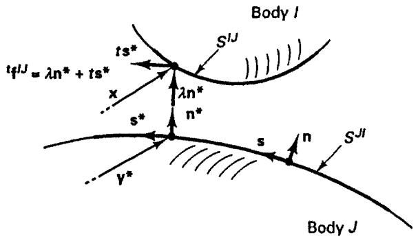Let $\mathbf{n}$ be the unit outward normal to $S^{JJ}$ and let $\mathbf{s}$ be a vector such that $\mathbf{n}$ , $\mathbf{s}$ form a right-hand basis (see Fig. 6.18). We can decompose the contact tractions $\mathbf{f}^{JJ}$ acting on $S^{JJ}$ into normal and tangential components corresponding to $\mathbf{n}$ and $\mathbf{s}$ on $S^{JJ}$ , $$ ^ {t} \mathbf {f} ^ {I J} = \lambda \mathbf {n} + t \mathbf {s} \tag {6.304} $$ where $\lambda$ and t are the normal and tangential traction components (for brevity of notation we do not use a superscript). Hence, $$ \lambda = (^ {t} \mathbf {f} ^ {I J}) ^ {T} \mathbf {n}; \quad t = (^ {t} \mathbf {f} ^ {I J}) ^ {T} \mathbf {s} \tag {6.305} $$ To define the actual values of $\mathbf{n}$ , $\mathbf{s}$ that we use in our contact calculations, consider a generic point $\mathbf{x}$ on $S^{JJ}$ and let $\mathbf{y}^{*}(\mathbf{x}, t)$ be the point on $S^{JJ}$ satisfying $$ \| \mathbf {x} - \mathbf {y} ^ {*} (\mathbf {x}, t) \| _ {2} = \min _ {\mathbf {y} \in S ^ {J I}} \{\| \mathbf {x} - \mathbf {y} \| _ {2} \} \tag {6.306} $$ The (signed) distance from $\mathbf{x}$ to $S^{J}$ is then given by $$ g (\mathbf {x}, t) = (\mathbf {x} - \mathbf {y} ^ {*}) ^ {T} \mathbf {n} ^ {*} \tag {6.307} $$ where $n^{*}$ is the unit “normal vector” that we use at $\mathbf{y}^{*}(\mathbf{x}, t)$ (see Fig. 6.18) and $n^{*}$ , $s^{*}$ are used in (6.304) corresponding to the point x. The function g is the gap function for the contact surface pair. 

text_image

Body I ts* S^IJ t f^IJ = λn* + ts* x λn* s* n* s n S^JI y* Body J

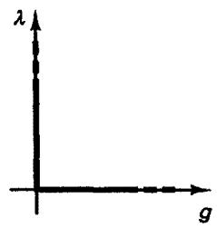
Figure 6.18 Definitions used in contact analysis With these definitions, the conditions for normal contact can now be written as $$ g \geq 0; \quad \lambda \geq 0; \quad g \lambda = 0 \tag {6.308} $$ where the last equation expresses the fact that if $g > 0$ , then we must have $\lambda = 0$ , and vice versa. To include frictional conditions, let us assume that Coulomb's law of friction holds pointwise on the contact surface and that $\mu$ is the coefficient of friction. This assumption means of course that frictional effects are included in a very simplified manner (for more details see, for example, E. Rabinowicz[A]). 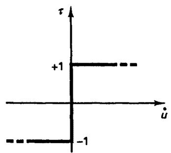Let us define the nondimensional variable $\tau$ given by $$ \tau = \frac {t}{\mu \lambda} \tag {6.309} $$ where $\mu\lambda$ is the “frictional resistance,” and the magnitude of the relative tangential velocity $$ \dot {u} (\mathbf {x}, t) = \left(\dot {\mathbf {u}} ^ {J} \right| _ {\mathbf {y} ^ {*} (\mathbf {x}, t)} - \left. \dot {\mathbf {u}} ^ {J} \right| _ {(\mathbf {x}, t)}) \cdot \mathbf {s} ^ {*} \tag {6.310} $$ corresponding to the unit tangential vector s at $\mathbf{y}^{*}(\mathbf{x}, t)$ . Hence, $\dot{u}(\mathbf{x}, t)\mathbf{s}^{*}$ is the tangential velocity at time t of the material point at $y^{*}$ relative to the material point at x. With these definitions Coulomb's law of friction states and $\left|\tau\right|\leq1$ $\left|\tau\right|<1$ implies $\dot{u}=0$ while $\left|\tau\right|=1$ implies sign $(\dot{u})=\text{sign }(\tau)$ (6.311) Figure 6.19 illustrates these interface conditions. The solution of the contact problem in Fig. 6.17 therefore entails the solution of the virtual work equation (6.301) (specialized for bodies I and J) subject to the conditions (6.308) and (6.311). 

text_image

λ g

Normal conditions 

text_image

τ +1 -1 û

Tangential conditions Figure 6.19 Interface conditions in contact analysis In the preceding equations, we considered in essence static (or pseudo-static) contact conditions. In dynamic analysis, the distributed body force includes the inertia force effects, and the kinematic interface conditions must be satisfied at all instances of time. Various algorithmic approaches for general contact analyses have been proposed, see P. Wriggers [A] and N. El-Abbasi and K. J. Bathe [A] and the references therein. In the simplest case, complete gluing is assumed and here different meshes are in essence glued firmly together. With proper mesh selections, although the meshes are quite different, full compatibility is achieved. With frictionless sliding and gap opening allowed, small displacement conditions are frequently assumed and the solution is considerably less complex than when large motions with frictional sliding, in statics or dynamics, are to be simulated. The changes in constraints and the possibility of ill-conditioning then require special attention, see for example K. J. Bathe and A. B. Chaudhary [B], G. Zavarise, P. Wriggers, and B. A. Schrefler [A], K. J. Bathe and P. A. Bouzinov [A], D. Pantuso, K. J. Bathe, and P. A. Bouzinov [A], and, for insight through a mathematical analysis, K. J. Bathe and F. Brezzi [C]. To exemplify the solution of contact problems, let us consider in the next section how the contact constraints are imposed in one solution approach (see also A. L. Eterovic and K. J. Bathe [C]). # 6.7.2 A Solution Approach for Contact Problems: # The Constraint Function Method Let w be a function of g and $\lambda$ such that the solutions of $w(g, \lambda) = 0$ satisfy the conditions (6.308), and similarly, let v be a function of $\tau$ and $\dot{u}$ such that the solutions of $v(\dot{u}, \tau) = 0$ satisfy the conditions (6.311). Then the contact conditions are given by $$ w (g, \lambda) = 0 \tag {6.312} $$ and $v(\dot{u},\tau) = 0$ (6.313) These conditions can now be imposed on the principle of virtual work equation using either a penalty approach or a Lagrange multiplier method (see Section 3.4). The variables $\lambda$ and $\tau$ can be considered Lagrange multipliers, and so we let $\delta\lambda$ and $\delta\tau$ be variations in these quantities (see Section 4.4.2). Multiplying (6.312) by $\delta \lambda$ and (6.313) by $\delta \tau$ and integrating over $S^{IJ}$ , we obtain the constraint equation $$ \int_ {S ^ {I J}} \left[ \delta \lambda w (g, \lambda) + \delta \tau v (\dot {u}, \tau) \right] d S ^ {I J} = 0 \tag {6.314} $$ In summary, the governing equations to be solved for the two-body contact problem in Fig. 6.17 are the usual principle of virtual work equation, with the effect of the contact tractions included through externally applied (but unknown) forces, plus the constraint equation (6.314). Of course, the principle of virtual work (6.301) is in the two-body contact problem specialized to bodies I and J only, and the contact force term is given by (6.302) and (6.303). The finite element solution of the governing continuum mechanics equations is obtained by using the discretization procedures for the principle of virtual work, and in addition now discretizing the contact conditions also. 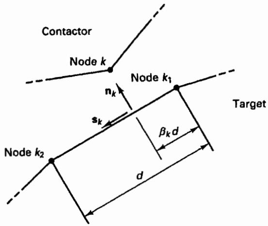To exemplify the formulation of the governing finite element equations, let us consider the two-dimensional case of contactor and target bodies shown schematically in Fig. 6.20. We notice that node $k_{1}$ and node $k_{2}$ define a straight boundary but are not necessarily the corner nodes of an element. Instead they are any adjacent nodes on the target body. The discretization of the continuum mechanics equations (6.301) and (6.314) corresponding to the conditions at time $t + \Delta t$ gives $$ { } ^ { t + \Delta t } \mathbf { F } ( { } ^ { t + \Delta t } \mathbf { U } ) = { } ^ { t + \Delta t } \mathbf { R } - { } ^ { t + \Delta t } \mathbf { R } _ { c } ( { } ^ { t + \Delta t } \mathbf { U } , { } ^ { t + \Delta t } \boldsymbol { \tau } ) \tag {6.315} $$ and $t+\Delta t\mathbf{F}_{c}(t+\Delta t\mathbf{U},t+\Delta t\tau)=0$ (6.316) where with m contactor nodes, $$ { } ^ { t + \Delta t } \boldsymbol { \tau } ^ { T } = \left[ \lambda _ { 1 } , \tau _ { 1 } , \dots , \lambda _ { k } , \tau _ { k } , \dots , \lambda _ { m } , \tau _ { m } \right] \tag {6.317} $$ Note that the relative velocity and gap functions are of course expressed in terms of the nodal point displacements. 

text_image

Contactor Node k n_k Node k_1 s_k β_k d Target Node k_2 d

Figure 6.20 Two-dimensional case of contact The vector $^{t+\Delta t}R_{c}$ is obtained by assembling for all m contactor nodes, $k = 1, \ldots, m$ , the nodal point force vectors due to contact. For the contactor node k and the corresponding target nodes, the nodal force vector is $$ { } ^ { t + \Delta t } \mathbf { R } _ { k } ^ { c } = \left[ \begin{array} { c } - \lambda _ { k } ( \mathbf { n } _ { k } + \mu \tau _ { k } \mathbf { s } _ { k } ) \\ ( 1 - \beta _ { k } ) \lambda _ { k } ( \mathbf { n } _ { k } + \mu \tau _ { k } \mathbf { s } _ { k } ) \\ \beta _ { k } \lambda _ { k } ( \mathbf { n } _ { k } + \mu \tau _ { k } \mathbf { s } _ { k } ) \end{array} \right] \tag {6.318} $$ where $\beta_{k},\mathbf{n}_{k},\mathbf{s}_{k}$ are defined in Fig. 6.20. The vector $t+\Delta tF_{c}$ can be written as $$ { } ^ { t + \Delta t } \mathbf { F } _ { c } ^ { T } = \left[ { } ^ { t + \Delta t } \mathbf { F } _ { 1 } ^ { c ^ { T } } , \dots , { } ^ { t + \Delta t } \mathbf { F } _ { m } ^ { c ^ { T } } \right] \tag {6.319} $$ where $t + \Delta t\mathbf{F}_k^c = \begin{bmatrix} w(g_k,\lambda_k)\\ v(\dot{u}_k,\tau_k) \end{bmatrix}$ (6.320) The incremental equations for solution of (6.315) and (6.316) are obtained by linearization about the last calculated state. Following the procedures discussed in Section 6.3.1, the resulting equations corresponding to the linearization about the state at time t are $$ \left[ \begin{array}{c c} \left(^ {t} \mathbf {K} + ^ {t} \mathbf {K} _ {u u} ^ {c}\right) & ^ {t} \mathbf {K} _ {u \tau} ^ {c} \\ ^ {t} \mathbf {K} _ {\tau u} ^ {c} & ^ {t} \mathbf {K} _ {\tau \tau} ^ {c} \end{array} \right] \left[ \begin{array}{l} \Delta \mathbf {U} \\ \Delta \boldsymbol {\tau} \end{array} \right] = \left[ \begin{array}{c} ^ {t + \Delta t} \mathbf {R} - ^ {t} \mathbf {F} - ^ {t} \mathbf {R} _ {c} \\ - ^ {t} \mathbf {F} _ {c} \end{array} \right] \tag {6.321} $$ where $\Delta \mathbf{U}$ and $\Delta \tau$ are the increments in the solution variables ${}^t\mathbf{U}$ and ${}^\prime \tau$ , and ${}^t\mathbf{K}_{uu}^c$ , ${}^t\mathbf{K}_{u\tau}^c$ , ${}^t\mathbf{K}_{\tau u}^c$ , and ${}^t\mathbf{K}_{\tau \tau}^c$ are contact stiffness matrices, $$ \left. \begin{array}{l} ^ {t} \mathbf {K} _ {u u} ^ {c} = \frac {\partial^ {t} \mathbf {R} _ {c}}{\partial^ {t} \mathbf {U}}; \quad {} ^ {t} \mathbf {K} _ {u \tau} ^ {c} = \frac {\partial^ {t} \mathbf {R} _ {c}}{\partial^ {t} \boldsymbol {\tau}} \\ ^ {t} \mathbf {K} _ {\tau u} ^ {c} = \frac {\partial^ {t} \mathbf {F} _ {c}}{\partial^ {t} \mathbf {U}}; \quad {} ^ {t} \mathbf {K} _ {\tau \tau} ^ {c} = \frac {\partial^ {t} \mathbf {F} _ {c}}{\partial^ {t} \boldsymbol {\tau}} \end{array} \right\} \tag {6.322} $$ The detailed expressions of these matrices depend on the actual constraint functions used. In practice, we use functions that very closely approximate the constraints shown in Fig. 6.19 but that are differentiable as required by the expressions in (6.322) (see Exercise 6.93). The continuum mechanics formulation in Section 6.7.1 has been given for very general conditions of deformations and constitutive relations (but Coulomb's law of friction was assumed). Of course, the formulation is also applicable to frictionless contact. In this case, only the constraint (6.308) needs to be imposed, and the finite element equations have only the normal forces at the contactor nodes as unknowns. Note that the coefficient matrix in (6.321) including frictional conditions is in general nonsymmetric, but a symmetric matrix can be obtained when friction is neglected. Of particular concern in the solution of contact problems is the capacity of the algorithm to converge when complex geometries, deformations, and contact conditions are analyzed. It should be noted here that although the incremental equations (6.321) correspond to a full linearization, the use of too large incremental steps may lead to convergence difficulties in the equilibrium iterations because the predicted intermediate state is too far from the solution. Also, full quadratic convergence when near the solution may not be observed when the change in the tangent coefficient matrix is not sufficiently smooth, for example, as a result of geometric kinks on the target surface. # 6.7.3 Exercises 6.91. Show that with the sign conventions used in (6.303) to (6.310) the statements of frictional contact in (6.308) and (6.311) are correct. 6.92. Consider frictionless contact between two bodies. Develop the general governing finite element equations with the imposition of the constraint function (6.312) using a penalty method (see Section 3.4.1). 6.93. The following constraint function $w(g, \lambda)$ for the constraint function algorithm is proposed $$ w (g, \lambda) = \frac {g + \lambda}{2} - \sqrt {\left(\frac {g - \lambda}{2}\right) ^ {2} + \epsilon} $$ where $\epsilon$ is very small but larger than zero. Plot this function for various values of $\epsilon$ and show that this $w(g, \lambda)$ is indeed a suitable function. 6.94. Design a function $v(\dot{u}, \tau)$ , as used in (6.313), to impose the frictional constraint given in (6.311). # 6.8 SOME PRACTICAL CONSIDERATIONS The establishment of an appropriate mathematical model for the analysis of an engineering problem is to a large degree based on sufficient understanding of the problem under consideration and a reasonable knowledge of the finite element procedures available for solution (see Section 1.2). This observation is particularly applicable in nonlinear analysis because the appropriate nonlinear kinematic formulations, material models, and solution strategies need to be selected. The objective in this section is to discuss briefly some important practical aspects pertaining to the selection of appropriate models and solution methods for nonlinear analysis. # 6.8.1 The General Approach to Nonlinear Analysis In an actual engineering analysis, it is good practice that a nonlinear analysis of a problem is always preceded by a linear analysis, so that the nonlinear analysis is considered an extension of the complete analysis process beyond the assumptions of linear analysis. Based on the linear response solution, the analyst is able to predict which nonlinearities will be significant and how to account for these nonlinearities most appropriately. Namely, the linear analysis results indicate the regions where geometric nonlinearities may be significant and where the material exceeds its elastic limit. Unfortunately, when performing a nonlinear analysis, there is frequently a tendency to select immediately a large number of elements and the most general nonlinear formulations available for modeling the problem. The engineering time used to prepare the model is large, the computer time that is needed for the analysis of the model is also very significant, and usually a voluminous amount of information is generated that cannot be fully absorbed and interpreted. If there are significant modeling or program input errors, it may also happen that the analyst “gives up in despair” during the course of the analysis because a relatively large amount of money has already been spent on the analysis, no significant results are as yet available, and the analyst is unable to realistically estimate how much further expense there would be until significant results could be produced. The important point is that such an approach to nonlinear analysis cannot be recommended. Instead, a linear model should first be established that contains important characteristics of the analysis problem. After some linear analyses have been performed that provide insight into the problem under consideration, the allowance for some nonlinearities—and not necessarily immediately for all nonlinearities that can be anticipated—should be made by choosing appropriate nonlinear formulations and material models. Here it should be noted that by employing the formulations discussed in Chapter 5 and this chapter, finite elements formulated using the linear analysis assumptions, the materially-nonlinear-only formulation, and the TL and UL formulations can all be used together in one finite element idealization. If this finite element mesh is a compatible mesh in linear analysis, the elements will also remain displacement-compatible in nonlinear analysis. The subdivision of the complete finite element idealization into elements governed by different nonlinear formulations merely means that in the analysis different nonlinearities are being accounted for in different parts of the structure. An effective procedure for introducing different kinds of nonlinearities into the analysis is the use of linear and nonlinear element groups. The complete process of analysis can be likened to a series of laboratory experiments in which different assumptions are made in each experiment—in the finite element analysis these experiments are performed on the computer with a finite element program. The advantages of starting with a linear analysis after which judiciously selected nonlinear analyses are performed are that, first, the effect of each nonlinearity introduced can more easily be explained, second, confidence in the analysis results can be established and, third, useful information is accumulated throughout the period of analysis. In addition to the general recommendations for an appropriate approach to nonlinear analysis given above, some practical aspects can be important and are briefly discussed in the following sections. # 6.8.2 Collapse and Buckling Analyses The objective of a nonlinear analysis is in many cases to estimate the maximum load that a structure can support prior to structural instability or collapse. In the analysis the load distribution on the structure is known, but the load magnitude that the structure can sustain is unknown. Figure 6.21 illustrates schematically the response of some structures that collapse or buckle. In each case, only the kinematic nonlinearities are considered, and the response would be different if material nonlinearities were also present. A thin plate does not have a collapse point; indeed because of membrane action, the plate increases its stiffness as the displacements grow. An arch, however, for specific geometric parameters, will collapse if the load increases. As shown in Fig. 6.21(a), the response beyond the collapse point A is referred to as the postbuckling behavior. In actuality, the response beyond point A, when induced by a load increase, is a dynamic response. However, the prediction of the (idealized) static postbuckling response can be important because, if the points A and $A'$ are very close to each other, then the collapse load corresponding to point A may not be as serious a restriction in the design although in general a dynamic response solution from point A onwards may be more appropriate. The response of the column depicted in Fig. 6.21(b) depends on the value of $\beta$ . This parameter represents the imperfection in the geometry and material properties of the column or the load application (from being exactly vertical). We note that the bifurcation buckling response of a perfectly straight column with only an end compressive load is approached as $\beta$ becomes very small. In all the analyses cases, however, the response can be calculated by an incremental analysis, provided the load can also decrease as the structural response dictates in the postbuckling regime. Hence, we should consider the following generic problem statement. Let $^{\Delta t}R$ be the vector which defines the load distribution. This vector corresponds to the first load step. Also, let $^{\tau}\beta$ be the load multiplier for any time $\tau$ to the load vector $^{\Delta t}R$ such that the load at time $\tau$ is $^{\tau}\beta^{\Delta t}R$ . In practice, we are frequently interested in calculating the response of the structure as $\tau$ increases. As illustrated in Fig. 6.21(a), this task requires that the load multiplier $^{\tau}\beta$ increase and decrease with $\tau$ as the structural response is calculated. We present a specific algorithm for the solution of the load multiplier $\tau\beta$ and the structural response in Section 8.4.3. With this solution method, the response of structures such as those shown in Fig. 6.21 is evaluated. However, the complete incremental nonlinear solution of a structure up to collapse and beyond can be expensive, and a linearized buckling analysis for the lowest buckling loads may be of value (see Section 3.2.3). The lowest calculated buckling load may be a reasonably good estimate of the actual collapse load (but only when the prebuckling displacements are small), and it may be important to use the buckling modes to define geometric imperfections of the structure. 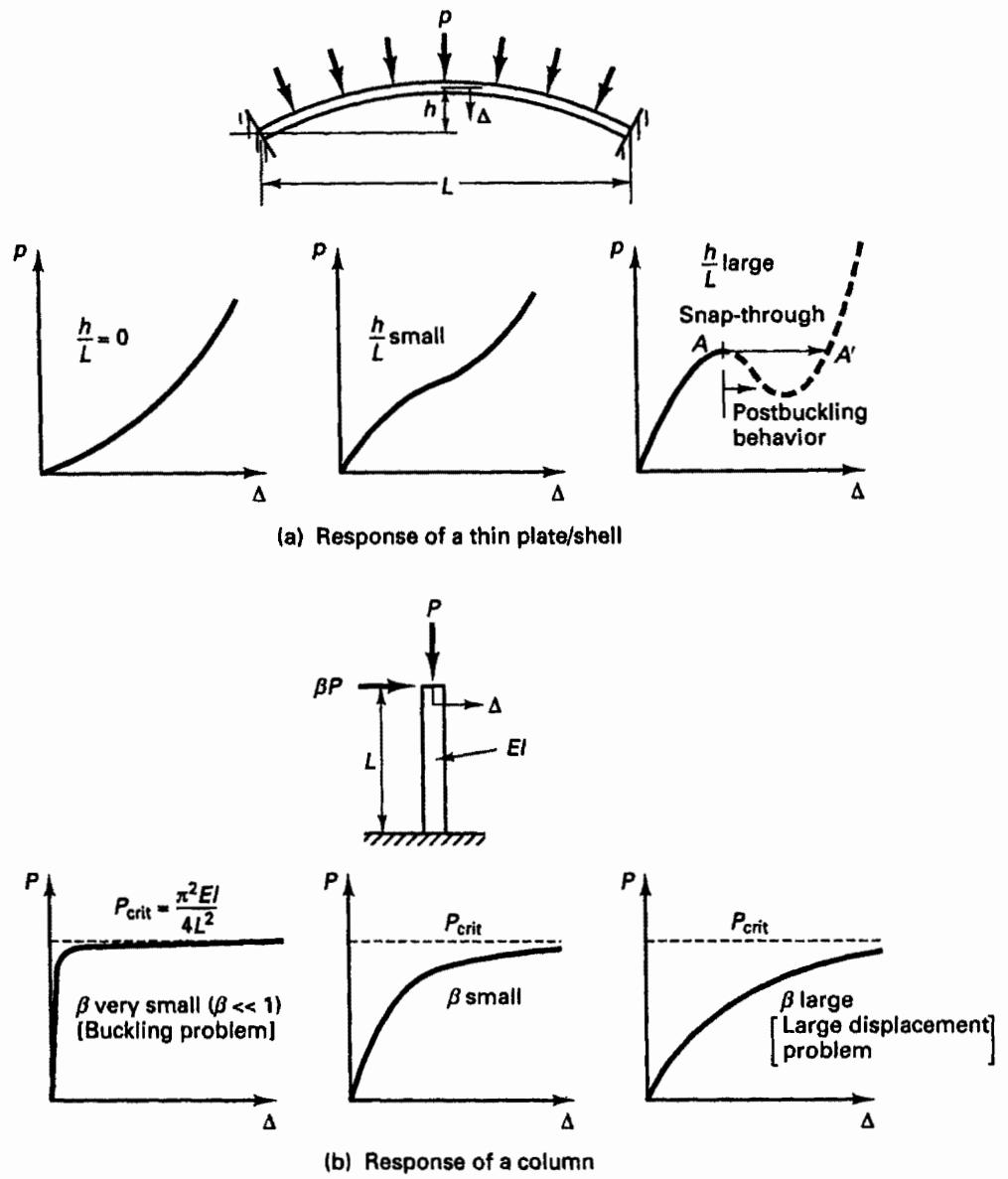That is, if imperfections that correspond to the lowest buckling modes are imposed on the “perfect” geometry of the structural model, the load-carrying capacity may be significantly reduced and be much more representative of  Figure 6.21 Instability and collapse analyses the load-carrying capacity of the actual physical structure (see the discussion of the analysis in Fig. 6.23). Let us consider the calculation of the linearized buckling load. The stiffness matrices at times $t - \Delta t$ and $t$ are $^{t - \Delta t}\mathbf{K}$ and $^t\mathbf{K}$ , and the corresponding vectors of externally applied loads are $^{t - \Delta t}\mathbf{R}$ and $^t\mathbf{R}$ . In the linearized buckling analysis, we assume that at any time $\tau$ , $$ \boxed {\tau \mathbf {K} = ^ {t - \Delta t} \mathbf {K} + \lambda (^ {t} \mathbf {K} - ^ {t - \Delta t} \mathbf {K})} \tag {6.323} $$ and $$ ^ {r} \mathbf {R} = ^ {t - \Delta t} \mathbf {R} + \lambda (^ {t} \mathbf {R} - ^ {t - \Delta t} \mathbf {R}) \tag {6.324} $$ where $\lambda$ is a scaling factor, and we are interested in those values of $\lambda$ that are greater than 1. At collapse or buckling the tangent stiffness matrix is singular, and hence, the condition for calculating $\lambda$ is $$ \det ^ {\tau} \mathbf {K} = 0 \tag {6.325} $$ or, equivalently (see Section 10.2), $$ ^ {\tau} \mathbf {K} \phi = \mathbf {0} \tag {6.326} $$ where $\phi$ is a nonzero vector. Substituting from (6.323) into (6.326), we obtain the eigenproblem $$ ^ {t - \Delta t} \mathbf {K} \phi = \lambda (^ {t - \Delta t} \mathbf {K} - ^ {t} \mathbf {K}) \phi \tag {6.327} $$ The eigenvalues $\lambda_{i}, i = 1, \ldots, n$ give the buckling loads [by using (6.324)], and the eigenvectors $\phi_{i}$ represent the corresponding buckling modes. We assume that the matrices 'K and '−Δ'K are both positive definite but note that in general '−Δ'K − 'K is indefinite; hence, the eigenproblem will have both positive and negative solutions (i.e., some eigenvalues will be negative). We are interested in only the smallest positive eigenvalues and therefore rewrite (6.327) as $$ { } ^ { t } \mathbf { K } \boldsymbol { \phi } = \gamma ^ { t - \Delta t } \mathbf { K } \boldsymbol { \phi } \tag {6.328} $$ where $$ \gamma = \frac {\lambda - 1}{\lambda} \tag {6.329} $$ The eigenvalues $\gamma_{i}$ in (6.328) are all positive, and usually only the smallest values $\gamma_{1}, \gamma_{2}, \ldots$ , are of interest. Namely, $\gamma_{1}$ corresponds to the smallest positive value of $\lambda$ in the problem (6.327). An important consideration is that the standard eigensolution techniques presented in Chapter 11 can be employed directly to solve for the smallest eigenvalues and corresponding vectors in (6.328) because both matrices in (6.328) are assumed to be positive definite. However, (6.329) shows that the eigenvalues $\gamma_{i}$ may be very closely spaced so that an effective shifting strategy may be important (see Sections 10.2.3 and 11.2.3). Having evaluated $\gamma_{1}$ , we obtain $\lambda_{1}$ from (6.329), and then the buckling (or collapse) load is given by (6.324), $$ \mathbf {R} _ {\text { buckling }} = ^ {t - \Delta t} \mathbf {R} + \lambda_ {1} (^ {t} \mathbf {R} - ^ {t - \Delta t} \mathbf {R}) \tag {6.330} $$ Similarly, we can evaluate the linearized buckling loads corresponding to $\gamma_{i}, i > 1$ . In practice, most frequently, the times $t - \Delta t$ and $t$ correspond to the times 0 (initial configuration with $^0\mathbf{R} = \mathbf{0}$ ) and $\Delta t$ (the first load step with $^{\Delta t}\mathbf{R}$ ). However, the above equations are applicable to any load step prior to collapse. Also, the relations (6.323) and (6.324) show that this analysis can be performed equally well when geometric or material nonlinearities are considered. 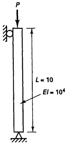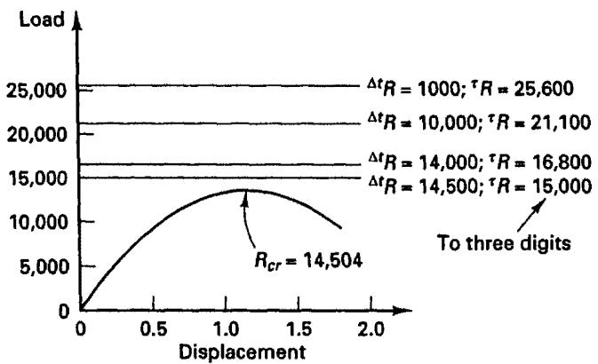The assumptions used in the linearized buckling analysis are displayed in (6.323) and (6.324); namely, we assume that the elements in the stiffness matrix vary linearly from time $t - \Delta t$ onward, the slope of the change being given by the difference from time $t - \Delta t$ to time t. The linearized buckling analysis therefore gives a reasonable estimate of the collapse load only if the precollapse displacements are relatively small (and any changes in the material properties are not significantly violating the assumption of linearity). Figure 6.22 gives the results of two analyses that illustrate this observation. In the analysis of the column, the prebuckling displacements are negligible and excellent results are obtained. On 

text_image

P L = 10 EI = 10^4

$P_{cr}$ of mathematical model (analytical solution) = 986.96 $P_{cr}$ of finite element model = 986.212 (for $\Delta tP = 1, 10$ , and 100) (a) Linearized buckling analysis of column; two Hermitian beam elements discussed in K. J. Bathe and S. Bolourchi [A] are used to model the column 

line

| ΔtR | τR | |-------|--------| | 1000 | 25,600 | | 10,000| 21,100 | | 14,000| 16,800 | | 14,500| 15,000 | | R_cr | 14,504 |

(b) Linearized buckling analysis of arch in Fig. E6.3; $L = 10$ ; $EA = 2.1 \times 10^{6}$ Figure 6.22 Linearized buckling analyses of two structures; in each case time $t-\Delta t$ corresponds to time 0 (the unstressed state).