text_image

20 kip 10 kip 2 3 4 100 kip-ft 1 5 10 ft 10 ft 10 ft 10 ft

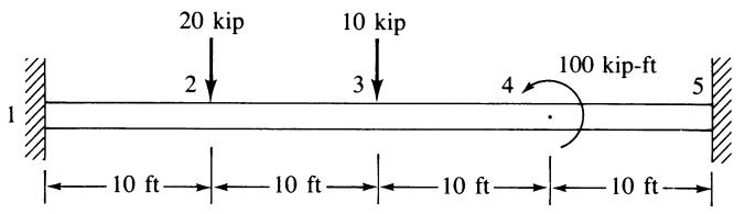
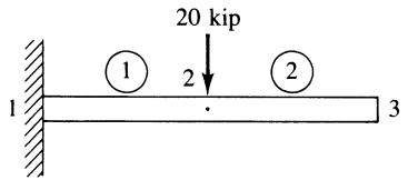
Figure 5–33 Beam analyzed by substructuring 

text_image

20 kip 1 2 2 3

Substructure 1 

text_image

10 kip 3 4 100 kip-ft 5

Substructure 2 Figure 5–34 Beam of Figure 5–33 separated into substructures The stiffness matrix for each beam element is given by Eq. (4.1.14) as $$ \begin{array}{l} \begin{array}{c c c} & 1 & 2 \\ & 2 & 3 \\ & 3 & 4 \\ & 4 & 5 \end{array} \\ \underline {{k}} ^ {(1)} = \underline {{k}} ^ {(2)} = \underline {{k}} ^ {(3)} = \underline {{k}} ^ {(4)} = \frac {2 9 \times 1 0 ^ {6}}{(1 2 0) ^ {3}} \left[ \begin{array}{c c c c} 1 2 & 6 (1 2 0) & - 1 2 & 6 (1 2 0) \\ 6 (1 2 0) & 4 (1 2 0) ^ {2} & - 6 (1 2 0) & 2 (1 2 0) ^ {2} \\ - 1 2 & - 6 (1 2 0) & 1 2 & - 6 (1 2 0) \\ 6 (1 2 0) & 2 (1 2 0) ^ {2} & - 6 (1 2 0) & 4 (1 2 0) ^ {2} \end{array} \right] (5.6.13) \\ = 1 6. 7 8 \left[ \begin{array}{c c c c} 1 2 & 7 2 0 & - 1 2 & 7 2 0 \\ 7 2 0 & 5 7, 6 0 0 & - 7 2 0 & 2 8, 8 0 0 \\ - 1 2 & - 7 2 0 & 1 2 & - 7 2 0 \\ 7 2 0 & 2 8, 8 0 0 & - 7 2 0 & 5 7, 6 0 0 \end{array} \right] (5.6.14) \\ \end{array} $$ For substructure 1, we add the stiffness matrices of elements 1 and 2 together. The equations are $$ 1 6. 7 8 \left[ \begin{array}{c c c c} 1 2 + 1 2 & - 7 2 0 + 7 2 0 & - 1 2 & 7 2 0 \\ - 7 2 0 + 7 2 0 & 5 7, 6 0 0 + 5 7, 6 0 0 & - 7 2 0 & 2 8, 8 0 0 \\ \hline - 1 2 & - 7 2 0 & 1 2 & - 7 2 0 \\ 7 2 0 & 2 8, 8 0 0 & - 7 2 0 & 5 7, 6 0 0 \end{array} \right] \left\{ \begin{array}{l} d _ {2 y} \\ \phi_ {2} \\ d _ {3 y} \\ \phi_ {3} \end{array} \right\} = \left\{ \begin{array}{c} - 2 0 \\ 0 \\ - 0 \\ 0 \end{array} \right\} \tag {5.6.15} $$ where the boundary conditions $d _ { 1 y } = \phi _ { 1 } = 0$ were used to reduce the equations. Rewriting Eq. (5.6.15) with the interface displacements first allows us to use Eq. (5.6.6) to condense out, or eliminate, the interior degrees of freedom, $d_{2y}$ and $\phi_{2}$ . These reordered equations are $$ \begin{array}{l} 1 6. 7 8 (1 2 d _ {3 y} - 7 2 0 \phi_ {3} - 1 2 d _ {2 y} - 7 2 0 \phi_ {2}) \quad = 0 \\ 1 6. 7 8 \left(- 7 2 0 d _ {3 y} + 5 7, 6 0 0 \phi_ {3} + 7 2 0 d _ {2 y} + 2 8, 8 0 0 \phi_ {2}\right) = 0 \tag {5.6.16} \\ 1 6. 7 8 \left(- 1 2 d _ {3 y} + 7 2 0 \phi_ {3} + 2 4 d _ {2 y} + \phi_ {2}\right) = - 2 0 \\ 1 6. 7 8 \left(- 7 2 0 d _ {2 y} + 2 8, 8 0 0 \phi_ {3} + 0 d _ {2 y} + 1 1 5, 2 0 0 \phi_ {2}\right) = 0 \\ \end{array} $$ Using Eq. (5.6.6), we obtain equations for the interface degrees of freedom as $$ \begin{array}{l} 1 6. 7 8 \left\{\left[ \begin{array}{c c} 1 2 & - 7 2 0 \\ - 7 2 0 & 5 7, 6 0 0 \end{array} \right] - \left[ \begin{array}{c c} - 1 2 & - 7 2 0 \\ 7 2 0 & 2 8, 8 0 0 \end{array} \right] \left[ \begin{array}{c c} 2 4 & 0 \\ 0 & 1 1 5, 2 0 0 \end{array} \right] ^ {- 1} \left[ \begin{array}{c c} - 1 2 & 7 2 0 \\ - 7 2 0 & 2 8, 8 0 0 \end{array} \right] \right\} \left\{ \begin{array}{c} d _ {3 y} \\ \phi_ {3} \end{array} \right\} \\ = \left\{ \begin{array}{l} 0 \\ 0 \end{array} \right\} - \left[ \begin{array}{c c} - 1 2 & - 7 2 0 \\ 7 2 0 & 2 8, 8 0 0 \end{array} \right] \left[ \begin{array}{c c} 2 4 & 0 \\ 0 & 1 1 5, 2 0 0 \end{array} \right] ^ {- 1} \left\{ \begin{array}{c} - 2 0 \\ 0 \end{array} \right\} \tag {5.6.17} \\ \end{array} $$ Simplifying Eq. (5.6.17), we obtain $$ \left[ \begin{array}{c c} 2 5. 1 7 & - 3 0 2 0 \\ - 3 0 2 0 & 4 8 3, 2 6 4 \end{array} \right] \left\{ \begin{array}{l} d _ {3 y} \\ \phi_ {3} \end{array} \right\} = \left\{ \begin{array}{l} - 1 0 \\ 6 0 0 \end{array} \right\} \tag {5.6.18} $$ For substructure 2, we add the stiffness matrices of elements 3 and 4 together. The equations are $$ 1 6. 7 8 \left[ \begin{array}{c c c c} 1 2 & 7 2 0 & - 1 2 & 7 2 0 \\ 7 2 0 & 5 7, 6 0 0 & - 7 2 0 & 2 8, 8 0 0 \\ - 1 2 & - 7 2 0 & 1 2 + 1 2 & - 7 2 0 + 7 2 0 \\ 7 2 0 & 2 8, 8 0 0 & - 7 2 0 + 7 2 0 & 5 7, 6 0 0 + 5 7, 6 0 0 \end{array} \right] \left\{ \begin{array}{l} d _ {3 y} \\ \phi_ {3} \\ d _ {4 y} \\ \phi_ {4} \end{array} \right\} = \left\{ \begin{array}{c} - 1 0 \\ 0 \\ 0 \\ 1 2 0 0 \end{array} \right\} \tag {5.6.19} $$ where boundary conditions $d_{5y} = \phi_{5} = 0$ were used to reduce the equations. Using static condensation, Eq. (5.6.6), we obtain equations with only the interface displacements $d_{3y}$ and $\phi_{3}$ . These equations are $$ \begin{array}{l} 1 6. 7 8 \left\{\left[ \begin{array}{c c} 1 2 & 7 2 0 \\ 7 2 0 & 5 7, 6 0 0 \end{array} \right] - \left[ \begin{array}{c c} - 1 2 & 7 2 0 \\ - 7 2 0 & 2 8, 8 0 0 \end{array} \right] \left[ \begin{array}{c c} 2 4 & 0 \\ 0 & 1 1 5, 2 0 0 \end{array} \right] ^ {- 1} \left[ \begin{array}{c c} - 1 2 & - 7 2 0 \\ 7 2 0 & 2 8, 8 0 0 \end{array} \right] \right\} \left\{ \begin{array}{c} d _ {3 y} \\ \phi_ {3} \end{array} \right\} \\ = \left\{ \begin{array}{c} - 1 0 \\ 0 \end{array} \right\} - \left[ \begin{array}{c c} - 1 2 & 7 2 0 \\ - 7 2 0 & 2 8, 8 0 0 \end{array} \right] \left[ \begin{array}{c c} 2 4 & 0 \\ 0 & 1 1 5, 2 0 0 \end{array} \right] ^ {- 1} \left\{ \begin{array}{c} 0 \\ 1 2 0 0 \end{array} \right\} \tag {5.6.20} \\ \end{array} $$ Simplifying Eq. (5.6.20), we obtain $$ \left[ \begin{array}{c c} 2 5. 1 7 & 3 0 2 0 \\ 3 0 2 0 & 4 8 3, 2 6 4 \end{array} \right] \left\{ \begin{array}{l} d _ {3 y} \\ \phi_ {3} \end{array} \right\} = \left\{ \begin{array}{l} - 1 7. 5 \\ - 3 0 0 \end{array} \right\} \tag {5.6.21} $$ Adding Eqs. (5.6.18) and (5.6.21), we obtain the final nodal equilibrium equations at the interface degrees of freedom as $$ \left[ \begin{array}{c c} 5 0. 3 4 & 0 \\ 0 & 9 6 6, 5 2 8 \end{array} \right] \left\{ \begin{array}{l} d _ {3 y} \\ \phi_ {3} \end{array} \right\} = \left\{ \begin{array}{l} - 2 7. 5 \\ 3 0 0 \end{array} \right\} \tag {5.6.22} $$ Solving Eq. (5.6.22) for the displacement and rotation at node 3, we obtain $$ d _ {3 y} = - 0. 5 4 6 3 \text { in. } \tag {5.6.23} $$ $$ \phi_ {3} = 0. 0 0 0 3 1 0 4 \mathrm{rad} $$ We could now return to Eq. (5.6.15) or Eq. (5.6.16) to obtain $d _ { 2 y }$ and $\phi _ { 2 }$ and to Eq. (5.6.19) to obtain $d _ { 4 y }$ and $\phi _ { 4 }$ . We emphasize that this example is used as a simple illustration of substructuring and is not typical of the size of problems where substructuring is normally performed. Generally, substructuring is used when the number of degrees of freedom is very large, as might occur, for instance, for very large structures such as the airframe in Figure 5–31. # References [1] Kassimali, A., Structural Analysis, 2nd ed., Brooks/Cole Publishers, Pacific Grove, CA, 1999. [2] Budynas, R. G., Advanced Strength and Applied Stress Analysis, 2nd ed., McGraw-Hill, New York, 1999. [3] Allen, H. G., and Bulson, P. S., Background to Buckling, McGraw-Hill, London, 1980. [4] Roark, R. J., and Young, W. C., Formulas for Stress and Strain, 6th ed., McGraw-Hill, New York, 1989. [5] Gere, J. M., Mechanics of Materials, 5th ed., Brooks/Cole Publishers, Pacific Grove, CA, 2001. [6] Parakh, Z. K., Finite Element Analysis of Bus Frames under Simulated Crash Loadings, M.S. Thesis, Rose-Hulman Institute of Technology, Terre Haute, Indiana, May 1989. [7] Martin, H. C., Introduction to Matrix Methods of Structural Analysis, McGraw-Hill, New York, 1966. [8] Juvinall, R. C., and Marshek, K. M., Fundamentals of Machine Component Design, 4th ed., p. 198, Wiley, 2005. # Problems # Solve all problems using the finite element stiffness method. 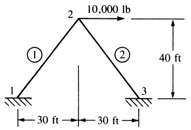5.1 For the rigid frame shown in Figure P5–1, determine (1) the displacement components and the rotation at node 2, (2) the support reactions, and (3) the forces in each element. Then check equilibrium at node 2. Let $E = 3 0 \times 1 0 ^ { 6 }$ psi, $A = 1 0 { \mathrm { ~ i n } } ^ { 2 } $ , and $I = 5 0 0 \mathrm { i n } ^ { 4 }$ for both elements. 

text_image

10,000 lb 2 ① ② 40 ft 1 30 ft 30 ft

Figure P5–1 

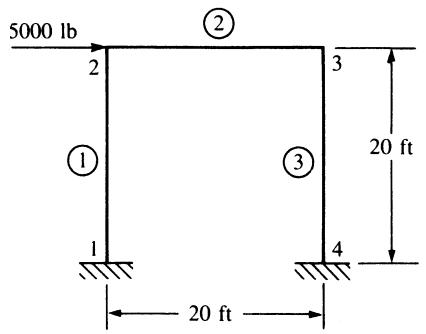
text_image

5000 lb ② 2 3 ① ③ 20 ft 1 4 20 ft

Figure P5–2 5.2 For the rigid frame shown in Figure P5–2, determine (1) the nodal displacement components and rotations, (2) the support reactions, and (3) the forces in each element. Let $E = 3 0 \times 1 0 ^ { 6 }$ psi, $\dot { A } = 1 0 \mathrm { i n } ^ { \bar { 2 } } ;$ , and $I = 2 0 0 \mathrm { i n } ^ { 4 }$ for all elements. 5.3 For the rigid stairway frame shown in Figure P5–3, determine (1) the displacements at node 2, (2) the support reactions, and (3) the local nodal forces acting on each element. Draw the bending moment diagram for the whole frame. Remember that the angle between elements 1 and 2 is preserved as deformation takes place; similarly for the angle between elements 2 and 3. Furthermore, owing to symmetry, $d _ { 2 x } = - d _ { 3 x }$ , $d _ { 2 y } = d _ { 3 y }$ , and $\phi _ { 2 } = - \phi _ { 3 }$ . What size A36 steel channel section would be needed to keep the allowable bending stress less than two-thirds of the yield stress? (For A36 steel, the yield stress is 36,000 psi.) 

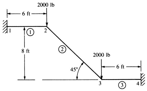
text_image

2000 lb 6 ft 1 ① 2 8 ft ② 45° 2000 lb 6 ft 3 ③ 4

Figure P5–3 5.4 For the rigid frame shown in Figure P5–4, determine (1) the nodal displacements and rotation at node 4, (2) the reactions, and (3) the forces in each element. Then check equilibrium at node 4. Finally, draw the shear force and bending moment diagrams for each element. Let $E = \stackrel { \cdot } { 3 } 0 \times 1 0 ^ { 3 }$ ksi, $A = 8 \ \mathrm { i n } ^ { 2 }$ , and $I = 8 0 0 ~ \mathrm { i n } ^ { 4 }$ for all elements. 

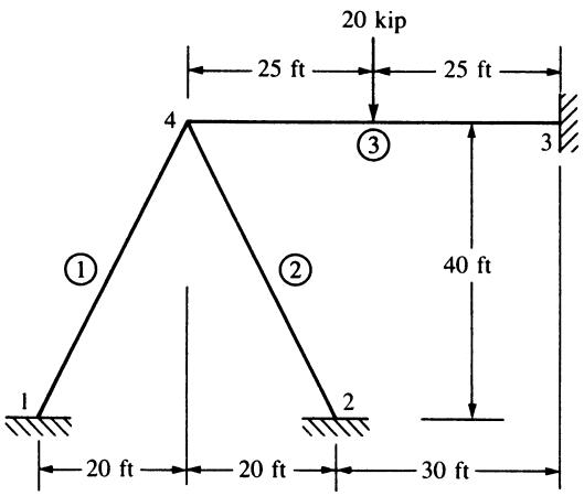
text_image

20 kip 25 ft 25 ft 4 ③ 3 ① ② 40 ft 1 2 2 2 2 30 ft

Figure P5–4 5.5–5.15 For the rigid frames shown in Figures P5–5—P5–15, determine the displacements and rotations of the nodes, the element forces, and the reactions. The values of E; A, and I to be used are listed next to each figure. 

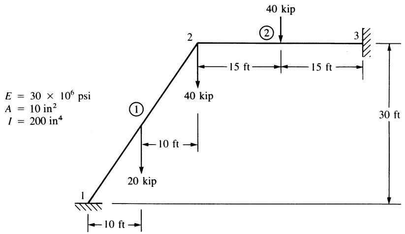
text_image

E = 30 × 10⁶ psi A = 10 in² I = 200 in⁴ 1 2 3 40 kip ② 15 ft 15 ft 40 kip 10 ft 20 kip 10 ft 30 ft

Figure P5–5 

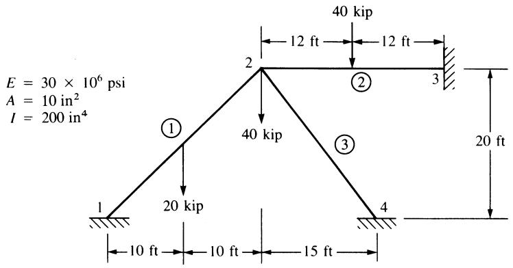
text_image

E = 30 × 10⁶ psi A = 10 in² I = 200 in⁴ 40 kip 12 ft 12 ft 2 ② 3 ① 40 kip ③ 20 ft 1 20 kip 4 10 ft 10 ft 15 ft

Figure P5–6 

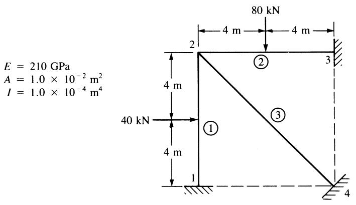
text_image

E = 210 GPa A = 1.0 × 10⁻² m² I = 1.0 × 10⁻⁴ m⁴ 80 kN 4 m 4 m 2 ② 3 4 m 40 kN ① ③ 4 m 1 4

Figure P5–7 

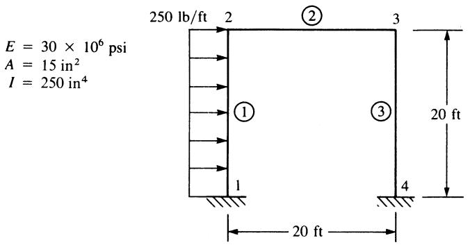
text_image

E = 30 × 10⁶ psi A = 15 in² I = 250 in⁴ 250 lb/ft 2 ② 3 ① ③ 1 4 20 ft 20 ft

Figure P5–8 

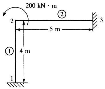
text_image

200 kN \u00b7 m 2 ② 5 m 3 ① 4 m 1

$$ \begin{array}{l} E = 2 1 0 \mathrm{GPa} \\ A = 2 \times 1 0 ^ {- 2} \mathrm{m} ^ {2} \\ I = 2 \times 1 0 ^ {- 4} \mathrm{m} ^ {4} \\ \end{array} $$ Figure P5-9 

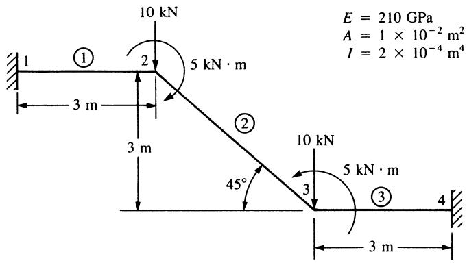
text_image

10 kN E = 210 GPa A = 1 × 10⁻² m² I = 2 × 10⁻⁴ m⁴ 1 ① 2 5 kN·m 3 m 3 m ② 10 kN 45° 5 kN·m 3 ③ 4 3 m

Figure P5-10 

text_image

2 20 kN ① ② 4 m 1 3 m 3 m 3

$$ \begin{array}{l} E = 7 0 \mathrm{GPa} \\ A = 3 \times 1 0 ^ {- 2} \mathrm{m} ^ {2} \\ I = 3 \times 1 0 ^ {- 4} \mathrm{m} ^ {4} \\ \end{array} $$ Figure P5-11 

text_image

3 m 1 100 kN ① ② 2 6 m 3

$$ E = 2 1 0 \mathrm{GPa} $$ $$ A = 8 \times 1 0 ^ {- 2} \mathrm{m} ^ {2} $$ $$ I = 1. 2 \times 1 0 ^ {- 4} \mathrm{m} ^ {4} $$ Figure P5–12 

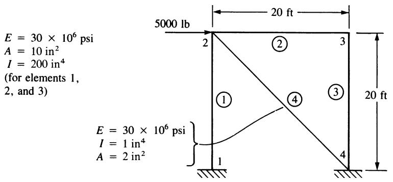
text_image

E = 30 × 10⁶ psi A = 10 in² I = 200 in⁴ (for elements 1, 2, and 3) 5000 lb 20 ft 2 ① ② ③ ④ ① ④ 20 ft E = 30 × 10⁶ psi I = 1 in⁴ A = 2 in² 1 4

Figure P5–13 

text_image

2000 lb/ft 10 ft 1 2 15 ft ② 3 45° ① E = 30 × 10⁶ psi A = 5 in² I = 200 in⁴

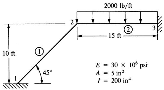
Figure P5–14 

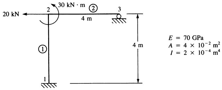
text_image

20 kN 2 30 kN·m ② 3 4 m ① 1 4 m E = 70 GPa A = 4 × 10⁻² m² I = 2 × 10⁻⁴ m⁴

Figure P5–15 5.16–5.18 Solve the structures in Figures P5–16—P5–18 by using substructuring. 

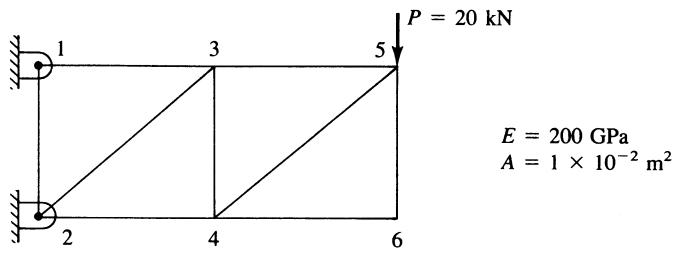
text_image

P = 20 kN E = 200 GPa A = 1 × 10⁻² m²

Figure P5–16 (Substructure the truss at nodes 3 and 4) 

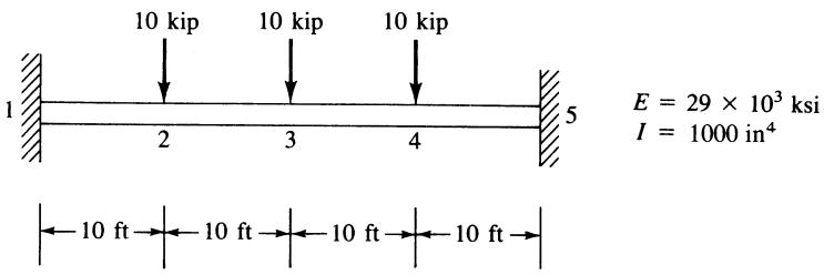
text_image

10 kip 10 kip 10 kip 1 2 3 4 5 E = 29 × 10³ ksi I = 1000 in⁴ 10 ft 10 ft 10 ft 10 ft

Figure P5–17 (Substructure the beam at node 3) 

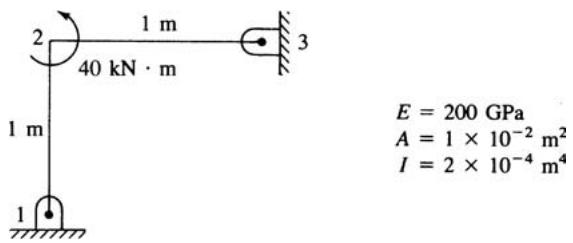
text_image

2 1 m 40 kN·m 1 m 1 3 E = 200 GPa A = 1 × 10⁻² m² I = 2 × 10⁻⁴ m⁴

Figure P5–18 (Substructure the beam at node 2) # Solve Problems 5.19–5.39 by using a computer program.  5.19 For the rigid frame shown in Figure P5–19, determine (1) the nodal displacement components and (2) the support reactions. (3) Draw the shear force and bending moment diagrams. For all elements, let $E = 3 0 \times 1 0 ^ { 6 } \mathrm { p s i } , I = 2 0 0 \mathrm { i n } ^ { 4 } .$ , and $A = 1 0 \mathrm { i n } ^ { 2 }$ . 

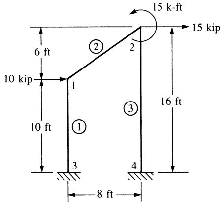
text_image

10 kip 6 ft 1 1 10 ft ① ② 2 ③ 15 k-ft 15 kip 16 ft 8 ft 3 4

Figure P5–19 

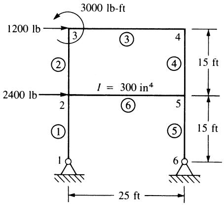
text_image

3000 lb-ft 1200 lb 3 ③ 4 ② ④ 2400 lb 2 2 I = 300 in⁴ 2 ⑥ 5 ① ⑤ 1 6 15 ft 15 ft 25 ft

Figure P5–20  5.20 For the rigid frame shown in Figure P5–20, determine (1) the nodal displacement components and (2) the support reactions. (3) Draw the shear force and bending moment diagrams. Let $E = \bar { 3 0 } \times 1 0 ^ { 6 } ~ \mathrm { p s i } , I = \bar { 2 0 } 0 ~ \mathrm { i n } ^ { 4 } .$ , and $A = 1 0 ~ \mathrm { i n } ^ { 2 }$ for all elements, except as noted in the figure.  5.21 For the slant-legged rigid frame shown in Figure P5–21, size the structure for minimum weight based on a maximum bending stress of 20 ksi in the horizontal beam elements and a maximum compressive stress (due to bending and direct axial load) of 15 ksi in the slant-legged elements. Use the same element size for the two slant-legged elements and the same element size for the two 10-foot sections of the horizontal element. Assume A36 steel is used. 

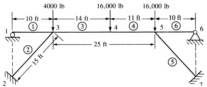
text_image

4000 lb 16,000 lb 16,000 lb 10 ft 14 ft 11 ft 10 ft ① ③ ④ ⑥ 1 3 4 5 25 ft ② 15 ft ⑤ 2 7

Figure P5–21  5.22 For the rigid building frame shown in Figure P5–22, determine the forces in each element and calculate the bending stresses. Assume all the vertical elements have $A = 1 0 { \mathrm { ~ i n } } ^ { 2 }$ and $I = 1 0 0 ~ \mathrm { i n } ^ { 4 }$ and all horizontal elements have $A = 1 5 { \mathrm { ~ i n } } ^ { 2 }$ and $I =$ $1 5 0 \ \mathrm { i n } ^ { 4 }$ . Let $E = 2 9 \times 1 0 ^ { 6 }$ psi for all elements. Let $c = 5$ in. for the vertical elements and $c = 6$ in. for the horizontal elements, where c denotes the distance from the