text_image

y 4 3 5 2 m 1 2 x 2 m

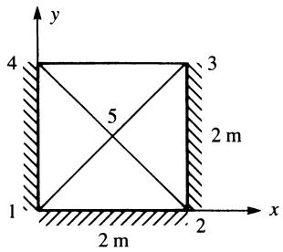
Figure 13–22 Discretized body of Figure 13–21 We will now calculate the element stiffness matrices. Because the magnitudes of the coordinates are the same as in Example 13.5, the element stiffness matrices are the same as Eqs. (13.5.23), (13.5.26), (13.5.28), and (13.5.30). Remember that there is no convection from any side of an element, so the convection contribution $[ k _ { h } ]$ to the stiffness matrix is zero. Superimposing the element stiffness matrices, we obtain the total stiffness matrix as $$ \underline {{{K}}} = \left[ \begin{array}{c c c c c} 2 5 & 0 & 0 & 0 & - 2 5 \\ 0 & 2 5 & 0 & 0 & - 2 5 \\ 0 & 0 & 2 5 & 0 & - 2 5 \\ 0 & 0 & 0 & 2 5 & - 2 5 \\ - 2 5 & - 2 5 & - 2 5 & - 2 5 & 1 0 0 \end{array} \right] \mathrm{W} / ^ {\circ} \mathrm{C} \tag {13.5.40} $$ Because the heat source $Q$ is acting uniformly over each element, we use Eq. (13.5.16) to evaluate the nodal forces for each element as $$ \left\{f ^ {(e)} \right\} = \frac {Q V}{3} \left\{ \begin{array}{l} 1 \\ 1 \\ 1 \end{array} \right\} = \frac {1 0 0 0 \left(1 \mathrm{m} ^ {3}\right)}{3} \left\{ \begin{array}{l} 1 \\ 1 \\ 1 \end{array} \right\} = \left\{ \begin{array}{l} 3 3 3 \\ 3 3 3 \\ 3 3 3 \end{array} \right\} \mathrm{W} \tag {13.5.41} $$ We then use Eqs. (13.5.40) and (13.5.41) applied to each element, to assemble the total system of equations as $$ \left[ \begin{array}{c c c c c} 2 5 & 0 & 0 & 0 & - 2 5 \\ 0 & 2 5 & 0 & 0 & - 2 5 \\ 0 & 0 & 2 5 & 0 & - 2 5 \\ 0 & 0 & 0 & 2 5 & - 2 5 \\ - 2 5 & - 2 5 & - 2 5 & - 2 5 & 1 0 0 \end{array} \right] \left\{ \begin{array}{l} t _ {1} \\ t _ {2} \\ t _ {3} \\ t _ {4} \\ t _ {5} \end{array} \right\} = \left\{ \begin{array}{c} 6 6 6 \\ 6 6 6 \\ 6 6 6 + F _ {3} \\ 6 6 6 + F _ {4} \\ 1 3 3 3 \end{array} \right\} \tag {13.5.42} $$ We have known nodal temperature boundary conditions of $t _ { 3 } = 1 0 0 ^ { \circ } \mathrm { C }$ and $t _ { 4 } =$ $1 0 0 ^ { \circ } \mathrm { C }$ . In the usual manner, as was shown in Example 13.4, we modify the stiffness and force matrices of Eq. (13.5.42) to obtain $$ \left[ \begin{array}{c c c c c} 2 5 & 0 & 0 & 0 & - 2 5 \\ 0 & 2 5 & 0 & 0 & - 2 5 \\ 0 & 0 & 1 & 0 & 0 \\ 0 & 0 & 0 & 1 & 0 \\ - 2 5 & - 2 5 & 0 & 0 & 1 0 0 \end{array} \right] \left\{ \begin{array}{l} t _ {1} \\ t _ {2} \\ t _ {3} \\ t _ {4} \\ t _ {5} \end{array} \right\} = \left\{ \begin{array}{l} 6 6 6 \\ 6 6 6 \\ 1 0 0 \\ 1 0 0 \\ 6 3 3 3 \end{array} \right\} \tag {13.5.43} $$ Equation (13.5.43) satisfies the boundary temperature conditions and is equivalent to Eq. (13.5.42); that is, the first, second, and fifth equations of Eq. (13.5.43) are the same as the first, second, and fifth equations of Eq. (13.5.42), and the third and fourth equations of Eq. (13.5.43) identically satisfy the boundary temperature conditions at nodes 3 and 4. The first, second, and fifth equations of Eq. (13.5.43) corresponding to the rows of unknown nodal temperatures, can now be solved simultaneously. The resulting solution is given by $$ t _ {1} = 1 8 0 ^ {\circ} \mathrm{C} \quad t _ {2} = 1 8 0 ^ {\circ} \mathrm{C} \quad t _ {5} = 1 5 3 ^ {\circ} \mathrm{C} \tag {13.5.44} $$ We then use the results from Eq. (13.5.44) in Eq. (13.5.42) to obtain the rates of heat flow at nodes 3 and 4 (that is, $F _ { 3 }$ and $F _ { 4 } )$ . # 13.6 Line or Point Sources A common practical heat-transfer problem is that of a source of heat generation present within a very small volume or area of some larger medium. When such heat sources exist within small volumes or areas, they may be idealized as line or point sources. Practical examples that can be modeled as line sources include hot-water pipes embedded within a medium such as concrete or earth, and conducting electrical wires embedded within a material. A line or point source can be considered by simply including a node at the location of the source when the discretized finite element model is created. The value of the line source can then be added to the row of the global force matrix corresponding to the global degree of freedom assigned to the node. However, another procedure can be used to treat the line source when it is more convenient to leave the source within an element. 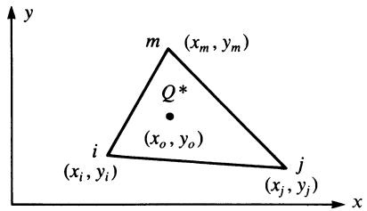We now consider the line source of magnitude $Q ^ { * }$ , with typical units of Btu/(h-ft), located at $\left( x _ { o } , y _ { o } \right)$ within the two-dimensional element shown in Figure 13–23. The heat source Q is no longer constant over the element volume. 

text_image

y m (xₘ, yₘ) Q* (xₒ, yₒ) i (xᵢ, yᵢ) j (xⱼ, yⱼ) x

Figure 13–23 Line source located within a typical triangular element Using Eq. (13.4.16), we can express the heat source matrix as $$ \left\{f _ {Q} \right\} = \iiint_ {V} \left\{ \begin{array}{l} N _ {i} \\ N _ {j} \\ N _ {m} \end{array} \right\} \Bigg | _ {x = x _ {o}, y = y _ {o}} \frac {Q ^ {*}}{A ^ {*}} d V \tag {13.6.1} $$ where $A ^ { * }$ is the cross-sectional area over which $Q ^ { * }$ acts, and the $N ^ { \star }$ s are evaluated at $x = x _ { o }$ and $\boldsymbol { y } = \boldsymbol { y } _ { o }$ . Equation (13.6.1) can be rewritten as $$ \left\{f _ {Q} \right\} = \iint_ {A ^ {*}} \int_ {0} ^ {t} \left\{ \begin{array}{l} N _ {i} \\ N _ {j} \\ N _ {m} \end{array} \right\} \Bigg | _ {x = x _ {o}, y = y _ {o}} \frac {Q ^ {*}}{A ^ {*}} d A d z \tag {13.6.2} $$ Because the $N { \mathrm { : } } $ are evaluated at $x = x _ { o }$ and $y = y _ { o } ,$ they are no longer functions of x and y. Thus, we can simplify Eq. (13.6.2) to $$ \left\{f _ {Q} \right\} = \left\{ \begin{array}{l} N _ {i} \\ N _ {j} \\ N _ {m} \end{array} \right\} \Bigg | _ {x = x _ {o}, y = y _ {o}} Q ^ {*} t \mathrm{Btu/h} \tag {13.6.3} $$ From Eq. (13.6.3), we can see that the portion of the line source $Q ^ { * }$ distributed to each node is based on the values of $N _ { i } , N _ { j } ,$ , and $N _ { m } .$ , which are evaluated using the coordinates $\left( x _ { o } , y _ { o } \right)$ of the line source. Recalling that the sum of the $N { \mathrm { : } } $ at any point within an element is equal to one [that is, $N _ { i } ( x _ { o } , y _ { o } ) + N _ { j } ( x _ { o } , y _ { o } ) + N _ { m } ( x _ { o } , y _ { o } ) = 1 ]$ , we see that no more than the total amount of $Q ^ { * }$ is distributed and that $$ Q _ {i} ^ {*} + Q _ {j} ^ {*} + Q _ {m} ^ {*} = Q ^ {*} \tag {13.6.4} $$ # Example 13.7 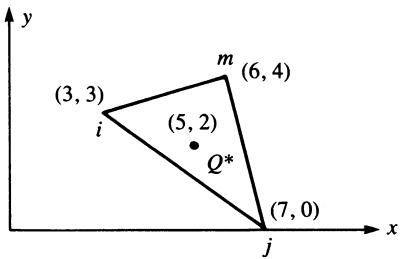A line source $Q ^ { * } = 6 5 ~ \mathrm { B t u } / ( \mathrm { h - i n . } )$ is located at coordinates ð5; 2Þ in the element shown in Figure 13–24. Determine the amount of $Q ^ { * }$ allocated to each node. All nodal coordinates are in units of inches. Assume an element thickness of $t = 1$ in. 

text_image

y (3, 3) i m (6, 4) (5, 2) Q* (7, 0) x j

Figure 13–24 Line source located within a triangular element We first evaluate the $\alpha _ { } ^ { } \mathrm { { s } } , \beta _ { } ^ { } \mathrm { { s } } ,$ , and $\gamma ^ { \prime } \mathbf { s } ,$ defined by Eqs. (6.2.10), associated with each shape function as follows: $$ \alpha_ {i} = x _ {j} y _ {m} - x _ {m} y _ {j} = 7 (4) - 6 (0) = 2 8 $$ $$ \alpha_ {j} = x _ {m} y _ {i} - x _ {i} y _ {m} = 6 (3) - 3 (4) = 6 $$ $$ \alpha_ {m} = x _ {i} y _ {j} - x _ {j} y _ {i} = 3 (0) - 7 (3) = - 2 1 $$ $$ \beta_ {i} = y _ {j} - y _ {m} = 0 - 4 = - 4 $$ $$ \beta_ {j} = y _ {m} - y _ {i} = 4 - 3 = 1 \tag {13.6.5} $$ $$ \beta_ {m} = y _ {i} - y _ {j} = 3 - 0 = 3 $$ $$ \gamma_ {i} = x _ {m} - x _ {j} = 6 - 7 = - 1 $$ $$ \gamma_ {j} = x _ {i} - x _ {m} = 3 - 6 = - 3 $$ $$ \gamma_ {m} = x _ {j} - x _ {i} = 7 - 3 = 4 $$ Also, $$ 2 A = \left| \begin{array}{c c c} 1 & x _ {i} & y _ {i} \\ 1 & x _ {j} & y _ {j} \\ 1 & x _ {m} & y _ {m} \end{array} \right| = \left| \begin{array}{c c c} 1 & 3 & 3 \\ 1 & 7 & 0 \\ 1 & 6 & 4 \end{array} \right| = 1 3 \tag {13.6.6} $$ Substituting the results of Eqs. (13.6.5) and (13.6.6) into Eq. (13.5.2) yields $$ N _ {i} = \frac {1}{1 3} [ 2 8 - 4 x - 1 y ] $$ $$ N _ {j} = \frac {1}{1 3} [ 6 + x - 3 y ] \tag {13.6.7} $$ $$ N _ {m} = \frac {1}{1 3} [ - 2 1 + 3 x + 4 y ] $$ Equations (13.6.7) for $N _ { i } , N _ { j }$ , and $N _ { m }$ evaluated at $x = 5$ and $y = 2$ are $$ N _ {i} = \frac {1}{1 3} [ 2 8 - 4 (5) - 1 (2) ] = \frac {6}{1 3} $$ $$ N _ {j} = \frac {1}{1 3} [ 6 + 5 - 3 (2) ] = \frac {5}{1 3} \tag {13.6.8} $$ $$ N _ {m} = \frac {1}{1 3} [ - 2 1 + 3 (5) + 4 (2) ] = \frac {2}{1 3} $$ Therefore, using Eq. (13.6.3), we obtain $$ \left\{ \begin{array}{l} f _ {Q i} \\ f _ {Q j} \\ f _ {Q m} \end{array} \right\} = Q ^ {*} t \left\{ \begin{array}{l} N _ {i} \\ N _ {j} \\ N _ {m} \end{array} \right\} _ {\substack {x = x _ {O} = 5 \\ y = y _ {O} = 2}} = \frac {6 5 (1)}{1 3} \left\{ \begin{array}{l} 6 \\ 5 \\ 2 \end{array} \right\} = \left\{ \begin{array}{l} 3 0 \\ 2 5 \\ 1 0 \end{array} \right\} \mathrm{Btu/h} \tag{13.6.9} $$ # 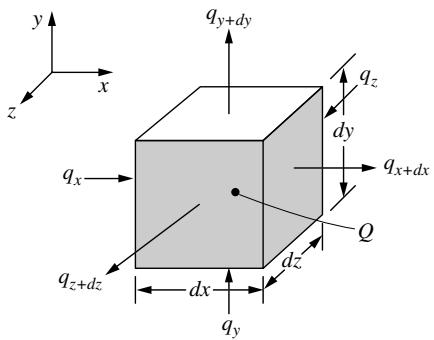d 13.7 Three-Dimensional Heat Transfer Finite Element Formulation When the heat transfer is in all three directions (indicated by $q _ { x } , q _ { y }$ and $q _ { z }$ in Figure 13–25), then we must model the system using three-dimensional elements to account for the heat transfer. Examples of heat transfer that often is three-dimensional are shown in Figure 13–26. Here we see in Figure 13–26(a) and (b) an electronic component soldered to a printed wiring board [11]. The model includes a silicon chip, silver-eutectic die, alumina carrier, solder joints, copper pads, and the printed wiring board. The model actually consisted of 965 8-noded brick elements with 1395 nodes and 216 thermal elements and was modeled in Algor [10]. One-quarter of the 

text_image

y x z qₓ qₓ+dy qₓ+dx qₓ+dz qₓ+dy qₓ qₓ+dy qₓ+dx qₓ qₓ+dy dx dz qᵧ

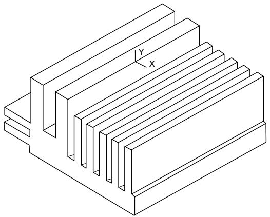
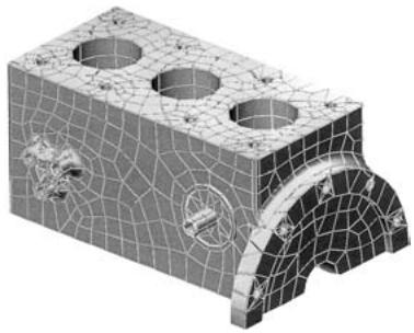
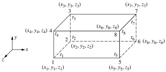
Figure 13–25 Three-dimensional heat transfer actual device was modeled. Figure 13–26(c) shows a heat sink used to cool a personal computer microprocessor chip (a two-dimensional model might possibly be used with good results as well). Finally, Figure 13–26(d) shows an engine block, which is an irregularly shaped three-dimensional body requiring a three-dimensional heat transfer analysis. The elements often included in commercial computer programs to analyze threedimensional heat transfer are the same as those used in Chapter 11 for threedimensional stress analysis. These include the four-noded tetrahedral (Figure 11–2), the eight-noded hexahedral (brick) (Figure 11–4), and the twenty-noded hexahedral (Figure 11–5), the difference being that we now have only one degree of freedom at each node, namely a temperature. The temperature functions in the x; y; and z directions can now be expressed by expanding Eq. (13.5.2) to the third dimension or by using shape functions given by Eq. (11.2.10) for a four-noded tetrahedral element or by Eqs. (11.3.3) for the eight-noded brick or the Eqs. (11.3.11)–(11.3.14) for the twenty-noded brick. The typical eight-noded brick element is shown in Figure 13–27 with the nodal temperatures included. 

natural_image

3D technical diagram of a microchip or integrated circuit grid with coordinate axes (X, Y, Z) and no visible text or symbols

FEA model of 68-pin SMT component (a) Electronic component soldered to printed circuit board 

natural_image

Isometric wireframe structure of a 3D geometric lattice (no text or symbols)

(b1) Carrier of the FEA model 

natural_image

Isometric diagram of a grid with a shaded cube overlay, no text or symbols present

(b2) Silicon chip (left side portion) and Au-Eutectic of FEA model 

natural_image

Isometric line drawing of a multi-tiered structural framework with no text or symbols

(b3) Solder joints and copper pads of FEA model 

natural_image

Isometric line drawing of a mechanical component or bracket (no text or symbols)

(b 4) Close-up of solder and copper pad (b) finite element model (quarter thermal model) showing the separate components 

natural_image

Isometric line drawing of a layered electronic component or circuit board structure (no text or symbols)

(c) Heat sink possibly used to cool a computer microchip 

natural_image

3D rendered mechanical component with grid pattern and circular holes (no text or symbols)

(d) Engine block Figure 13–26 Examples of three-dimensional heat transfer 

text_image

(x₃, y₃, z₃) (x₇, y₇, z₇) 3 7 t₃ (x₈, y₈, z₈) t₇ 4 (x₄, y₄, z₄) t₄ t₈ 2 t₂ 8 t₆ 6 (x₆, y₆, z₆) (x₂, y₂, z₂) t₁ t₅ 1 5 (x₁, y₁, z₁) (x₅, y₅, z₅) y x z

Figure 13–27 Eight-noded brick element showing nodal temperatures for heat transfer # 13.8 One-Dimensional Heat Transfer with Mass Transport We now consider the derivation of the basic differential equation for one-dimensional heat flow where the flow is due to conduction, convection, and mass transport (or transfer) of the fluid. The purpose of this derivation including mass transport is to show how Galerkin’s residual method can be directly applied to a problem for which the variational method is not applicable. That is, the differential equation will have an odd-numbered derivative and hence does not have an associated functional of the form of Eq. (1.4.3). 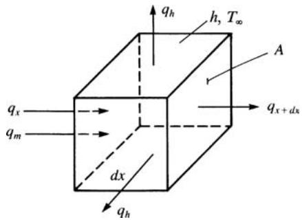The control volume used in the derivation is shown in Figure 13–28. Again, from Eq. (13.1.1) for conservation of energy, we obtain $$ q _ {x} A d t + Q A d x d t = c \rho A d x d T + q _ {x + d x} A d t + q _ {h} P d x d t + q _ {m} d t \tag {13.8.1} $$ All of the terms in Eq. (13.8.1) have the same meaning as in Sections 13.1 and 13.2, except the additional mass-transport term is given by [1] $$ q _ {m} = \dot {m} c T \tag {13.8.2} $$ where the additional variable m\_ is the mass flow rate in typical units of kg/h or slug/h. 

text_image

q_h h_3 T_\infty A r q_x q_m dx q_h q_{x+dx}

Figure 13–28 Control volume for onedimensional heat conduction with convection and mass transport Again, using Eqs. (13.1.3)–(13.1.6), (13.2.2), and (13.8.2) in Eq. (13.8.1) and differentiating with respect to x and t, we obtain $$ \frac {\partial}{\partial x} \left(K _ {x x} \frac {\partial T}{\partial x}\right) + Q = \frac {\dot {m} c}{A} \frac {\partial T}{\partial x} + \frac {h P}{A} (T - T _ {\infty}) + \rho c \frac {\partial T}{\partial t} \tag {13.8.3} $$ Equation (13.8.3) is the basic one-dimensional differential equation for heat transfer with mass transport. # 13.9 Finite Element Formulation of Heat Transfer with Mass Transport by Galerkin’s Method Having obtained the differential equation for heat transfer with mass transport, Eq. (13.8.3), we now derive the finite element equations by applying Galerkin’s residual method, as outlined in Section 3.12, directly to the differential equation. We assume here that Q = 0 and that we have steady-state conditions so that differentiation with respect to time is zero. The residual $R$ is now given by $$ R (T) = - \frac {d}{d x} \left(K _ {x x} \frac {d T}{d x}\right) + \frac {\dot {m} c}{A} \frac {d T}{d x} + \frac {h P}{A} (T - T _ {\infty}) \tag {13.9.1} $$ Applying Galerkin's criterion, Eq. (3.12.3), to Eq. (13.9.1), we have $$ \int_ {0} ^ {L} \left[ - \frac {d}{d x} \left(K _ {x x} \frac {d T}{d x}\right) + \frac {\dot {m} c}{A} \frac {d T}{d x} + \frac {h P}{A} (T - T _ {\infty}) \right] N _ {i} d x = 0 \quad (i = 1, 2) \tag {13.9.2} $$ where the shape functions are given by Eqs. (13.4.2). Applying integration by parts to the first term of Eq. (13.9.2), we obtain $$ u = N _ {i} \quad d u = \frac {d N _ {i}}{d x} d x \tag {13.9.3} $$ $$ d v = - \frac {d}{d x} \left(K _ {x x} \frac {d T}{d x}\right) d x \quad v = - K _ {x x} \frac {d T}{d x} $$ Using Eqs. (13.9.3) in the general formula for integration by parts [see Eq. (3.12.6)], we obtain $$ \int_ {0} ^ {L} \left[ - \frac {d}{d x} \left(K _ {x x} \frac {d T}{d x}\right) \right] N _ {i} d x = - K _ {x x} \frac {d T}{d x} N _ {i} \bigg | _ {0} ^ {L} + \int_ {0} ^ {L} K _ {x x} \frac {d T}{d x} \frac {d N _ {i}}{d x} d x \tag {13.9.4} $$ Substituting Eq. (13.9.4) into Eq. (13.9.2), we obtain $$ \int_ {0} ^ {L} \left(K _ {x x} \frac {d T}{d x} \frac {d N _ {i}}{d x}\right) d x + \int_ {0} ^ {L} \left[ \frac {\dot {m} c}{A} \frac {d T}{d x} + \frac {h P}{A} (T - T _ {\infty}) \right] N _ {i} d x = K _ {x x} \frac {d T}{d x} N _ {i} \Big | _ {0} ^ {L} \tag {13.9.5} $$ Using Eq. (13.4.2) in (13.4.1) for $T$ , we obtain $$ \frac {d T}{d x} = - \frac {t _ {1}}{L} + \frac {t _ {2}}{L} \tag {13.9.6} $$ From Eq. (13.4.2), we obtain $$ \frac {d N _ {1}}{d x} = - \frac {1}{L} \quad \frac {d N _ {2}}{d x} = \frac {1}{L} \tag {13.9.7} $$ By letting $N_{i}=N_{1}=1-(x/L)$ and substituting Eqs. (13.9.6) and (13.9.7) into Eq. (13.9.5), along with Eq. (13.4.1) for T, we obtain the first finite element equation $$ \begin{array}{l} \int_ {0} ^ {L} K _ {x x} \left(- \frac {t _ {1}}{L} + \frac {t _ {2}}{L}\right) \left(- \frac {1}{L}\right) d x + \int_ {0} ^ {L} \frac {\dot {m} c}{A} \left(- \frac {t _ {1}}{L} + \frac {t _ {2}}{L}\right) \left(1 - \frac {x}{L}\right) d x \\ + \int_ {0} ^ {L} \frac {h P}{A} \left[ \left(1 - \frac {x}{L}\right) t _ {1} + \left(\frac {x}{L}\right) t _ {2} - T _ {\infty} \right] \left(\frac {1 - x}{L}\right) d x = q _ {x 1} ^ {*} \tag {13.9.8} \\ \end{array} $$ where the definition for $q_{x}$ given by Eq. (13.1.3) has been used in Eq. (13.9.8). Equation (13.9.8) has a boundary condition $q_{x1}^{*}$ at x = 0 only because $N_{1} = 1$ at x = 0 and $N _ { 1 } = 0$ at x ¼ L. Integrating Eq. (13.9.8), we obtain $$ \left(\frac {K _ {x x} A}{L} - \frac {\dot {m} c}{2} + \frac {h P L}{3}\right) t _ {1} + \left(- \frac {K _ {x x} A}{L} + \frac {\dot {m} c}{2} + \frac {h P L}{6}\right) t _ {2} = q _ {x 1} ^ {*} + \frac {h P L}{2} T _ {\infty} \tag {13.9.9} $$ where $q _ { x 1 } ^ { * }$ is defined to be $q _ { x }$ evaluated at node 1. To obtain the second finite element equation, we let $N _ { i } = N _ { 2 } = x / L$ in Eq. (13.9.5) and again use Eqs. (13.9.6), (13.9.7), and (13.4.1) in Eq. (13.9.5) to obtain $$ \left(- \frac {K _ {x x} A}{L} - \frac {\dot {m} c}{2} + \frac {h P L}{6}\right) t _ {1} + \left(\frac {K _ {x x} A}{L} + \frac {\dot {m} c}{2} + \frac {h P L}{3}\right) t _ {2} = q _ {x 2} ^ {*} + \frac {h P L}{2} T _ {\infty} \tag {13.9.10} $$ where $q _ { x 2 } ^ { * }$ is defined to be $q _ { x }$ evaluated at node 2. Rewriting Eqs. (13.9.9) and (13.9.10) in matrix form yields $$ \begin{array}{l} \left[ \frac {K _ {x x} A}{L} \left[ \begin{array}{c c} 1 & - 1 \\ - 1 & 1 \end{array} \right] + \frac {\dot {m} c}{2} \left[ \begin{array}{c c} - 1 & 1 \\ - 1 & 1 \end{array} \right] + \frac {h P L}{6} \left[ \begin{array}{c c} 2 & 1 \\ 1 & 2 \end{array} \right] \right] \left\{ \begin{array}{c} t _ {1} \\ t _ {2} \end{array} \right\} \\ = \frac {h P L T _ {\infty}}{2} \left\{ \begin{array}{l} 1 \\ 1 \end{array} \right\} + \left\{ \begin{array}{l} q _ {x 1} ^ {*} \\ q _ {x 2} ^ {*} \end{array} \right\} \tag {13.9.11} \\ \end{array} $$ Applying the element equation $\{ f \} = [ k ] \{ t \}$ to Eq. (13.9.11), we see that the element stiffness (conduction) matrix is now composed of three parts: $$ [ k ] = [ k _ {c} ] + [ k _ {h} ] + [ k _ {m} ] \tag {13.9.12} $$ where $$ [ k _ {c} ] = \frac {K _ {x x} A}{L} \left[ \begin{array}{c c} 1 & - 1 \\ - 1 & 1 \end{array} \right] \quad [ k _ {h} ] = \frac {h P L}{6} \left[ \begin{array}{c c} 2 & 1 \\ 1 & 2 \end{array} \right] \quad [ k _ {m} ] = \frac {\dot {m} c}{2} \left[ \begin{array}{c c} - 1 & 1 \\ - 1 & 1 \end{array} \right] \tag {13.9.13} $$ and the element nodal force and unknown nodal temperature matrices are $$ \{f \} = \frac {h P L T _ {\infty}}{2} \left\{ \begin{array}{l} 1 \\ 1 \end{array} \right\} + \left\{ \begin{array}{l} q _ {x 1} ^ {*} \\ q _ {x 2} ^ {*} \end{array} \right\} \quad \{t \} = \left\{ \begin{array}{l} t _ {1} \\ t _ {2} \end{array} \right\} \tag {13.9.14} $$ We observe from Eq. (13.9.13) that the mass transport stiffness matrix $[ k _ { m } ]$ is asymmetric and, hence, ½k is asymmetric. Also, if heat flux exists, it usually occurs across the free ends of a system. Therefore, $q _ { x 1 }$ and $q _ { x 2 }$ usually occur only at the free ends of a system modeled by this element. When the elements are assembled, the heat fluxes $q _ { x 1 }$ and $q _ { x 2 }$ are usually equal but opposite at the node common to two elements, unless there is an internal concentrated heat flux in the system. Furthermore, for insulated ends, the $q _ { x } ^ { * } \mathbf { \bar { s } }$ also go to zero. To illustrate the use of the finite element equations developed in this section for heat transfer with mass transport, we will now solve the following problem. # Example 13.8 Air is flowing at a rate of 4.72 lb/h inside a round tube with a diameter of 1 in. and length of 5 in., as shown in Figure 13–29. The initial temperature of the air entering the tube is $1 0 0 ^ { \circ } \mathrm { F }$ . The wall of the tube has a uniform constant temperature of $2 0 0 ^ { \circ } \mathrm { F }$ . The specific heat of the air is 0.24 $\mathrm { B t u / ( l b \mathrm { - } ^ { \circ } F ) }$ , the convection coefficient 

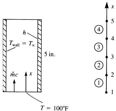
text_image

h Twall = T∞ 5 in. ṁc x T = 100°F x ④ 5 4 ③ 3 ② 2 ① 1

Figure 13–29 Air flowing through a tube, and the finite element model between the air and the inner wall of the tube is 2.7 Btu $/ ( \mathrm { h - f t } ^ { 2 } \mathrm { - } ^ { \circ } \mathrm { F } )$ , and the thermal conductivity is 0.017 $\mathrm { B t u / ( h \mathrm { - } f t \mathrm { - } ^ { \circ } F ) }$ . Determine the temperature of the air along the length of the tube and the heat flow at the inlet and outlet of the tube. Here the flow rate and specific heat are given in force units (pounds) instead of mass units (slugs). This is not a problem because the units cancel in the mc\_ product in the formulation of the equations. We first determine the element stiffness and force matrices using Eqs. (13.9.13) and (13.9.14). To do this, we evaluate the following factors: $$ \frac {K _ {x x} A}{L} = \frac {(0 . 0 1 7) \left[ \frac {\pi (1)}{4 (1 4 4)} \right]}{1 . 2 5 / 1 2} = 0. 8 9 1 \times 1 0 ^ {- 3} \mathrm{Btu} / (\mathrm{h} ^ {- \circ} \mathrm{F}) $$ $$ \dot {m} c = (4. 7 2) (0. 2 4) = 1. 1 3 3 \mathrm{Btu} / \left(\mathrm{h} ^ {- \circ} \mathrm{F}\right) \tag {13.9.15} $$ $$ \frac {h P L}{6} = \frac {(2 . 7) (0 . 2 6 2) (0 . 1 0 4)}{6} = 0. 0 1 2 3 \mathrm{Btu} / (\mathrm{h} ^ {- \circ} \mathrm{F}) $$ $$ h P L T _ {\infty} = (2. 7) (0. 2 6 2) (0. 1 0 4) (2 0 0) = 1 4. 7 1 \mathrm{Btu/h} $$ We can see from Eqs. (13.9.15) that the conduction portion of the stiffness matrix is negligible. Therefore, we neglect this contribution to the total stiffness matrix and obtain $$ \underline {{k}} ^ {(1)} = \frac {1 . 1 3 3}{2} \left[ \begin{array}{l l} - 1 & 1 \\ - 1 & 1 \end{array} \right] + 0. 0 1 2 3 \left[ \begin{array}{l l} 2 & 1 \\ 1 & 2 \end{array} \right] = \left[ \begin{array}{l l} - 0. 5 4 2 & 0. 5 7 9 \\ - 0. 5 5 4 & 0. 5 9 1 \end{array} \right] \tag {13.9.16} $$ Similarly, because all elements have the same properties, $$ \underline {{k}} ^ {(2)} = \underline {{k}} ^ {(3)} = \underline {{k}} ^ {(4)} = \underline {{k}} ^ {(1)} \tag {13.9.17} $$ Using Eqs. (13.9.14) and (13.9.15), we obtain the element force matrices as $$ \underline {{f}} ^ {(1)} = \underline {{f}} ^ {(2)} = \underline {{f}} ^ {(3)} = \underline {{f}} ^ {(4)} = \left\{ \begin{array}{l} 7. 3 5 \\ 7. 3 5 \end{array} \right\} \tag {13.9.18} $$