# Step 5 Solve for the velocity at time $t = 0 . 1$ s as $$ \begin{array}{l} \dot {d} _ {1} = 0 + (0. 1) \left[ \left(1 - \frac {1}{2}\right) (5 6. 5) + \left(\frac {1}{2}\right) (3 5. 4) \right] \\ \dot {d} _ {1} = 4. 5 9 \mathrm{in./s} \\ \end{array} $$ # Step 6 Repeated use of steps 3–5 will result in the displacement, acceleration, and velocity for additional time steps as desired. We will now perform one more time-step iteration. Repeating step 3 for the next time step $\left( t = 0 . 2 \ s \right)$ , we have $$ F _ {2} ^ {\prime} = 6 0 + \frac {1 . 7 7}{(\frac {1}{6}) (0 . 1) ^ {2}} \left[ 0. 2 4 8 + (0. 1) (4. 5 9) + \left(\frac {1}{2} - \frac {1}{6}\right) (0. 1) ^ {2} (3 5. 4) \right] $$ $$ F _ {2} ^ {\prime} = 9 3 4 \mathrm{lb} $$ $$ d _ {2} = \frac {9 3 4}{1 1 3 2} = 0. 8 2 5 \mathrm{in}. $$ Repeating step 4 for time step $t = 0 . 2 \ \mathrm { s } ,$ we obtain $$ \ddot {d} _ {2} = \frac {1}{(\frac {1}{6}) (0 . 1) ^ {2}} \left[ 0. 8 2 5 - 0. 2 4 8 - (0. 1) (4. 5 9) - (0. 1) ^ {2} \left(\frac {1}{2} - \frac {1}{6}\right) (3 5. 4) \right] $$ $$ \ddot {d} _ {2} = 1. 2 7 \mathrm {in. / s^ {2}} $$ Finally, repeating step 5 for time step $t = 0 . 2 \ \mathrm { s } ,$ we have $$ \dot {d} _ {2} = 4. 5 9 + (0. 1) \left[ \left(1 - \frac {1}{2}\right) (3 5. 4) + \frac {1}{2} (1. 2 7) \right] $$ $$ \dot {d} _ {2} = 6. 4 2 \mathrm{in./s} $$ Table 16–2 summarizes the results obtained through time $t = 0 . 5 \mathrm { ~ s ~ } .$ . Table 16–2 Results of the analysis of Example 16.2

t (s)	F(t) (lb)	di (in.)	Q (lb)	ddi (in./s2)	di (in./s)
0.	100	0	0	56.5	0
0.1	80	0.248	17.3	35.4	4.59
0.2	60	0.825	57.8	1.27	6.42
0.3	48.6	1.36	95.2	-26.2	5.17
0.4	45.7	1.72	120.4	-42.2	1.75
0.5	42.9	1.68	117.6	-42.2	-2.45

# Wilson’s Method We will now outline Wilson’s method (also called the Wilson-Theta method). Because of its general versatility, it has been adopted into the Algor computer program for purposes of structural dynamics analysis. Wilson’s method is an extension of the linear acceleration method wherein the acceleration is assumed to vary linearly within each time interval now taken from t to $t + \Theta \Delta t ,$ , where $\Theta \geqslant 1 . 0$ . For $\Theta = 1 . 0$ , the method reduces to the linear acceleration scheme. However, for unconditional stability in the numerical analysis, we must use $\Theta \geqslant 1 . 3 7 \left[ 7 , 8 \right]$ . In practice, $\Theta = 1 . 4 0$ is often selected. The Wilson equations are given in a form similar to the previous Newmark’s equations, Eqs. (16.3.9) and (16.3.10), as $$ \dot {d} _ {i + 1} = \dot {d} _ {i} + \frac {\Theta \Delta t}{2} (\ddot {d} _ {i + 1} + \ddot {d} _ {i}) \tag {16.3.15} $$ $$ d _ {i + 1} = d _ {i} + \Theta \Delta t \dot {d} _ {i} + \frac {\Theta^ {2} (\Delta t) ^ {2}}{6} (\ddot {d} _ {i + 1} + 2 \ddot {d} _ {i}) \tag {16.3.16} $$ where $\ddot { d } _ { i + 1 } , \dot { d } _ { i + 1 }$ , and $d _ { i + 1 }$ represent the acceleration, velocity, and displacement, respectively, at time $t + \Theta \Delta t$ . We seek a matrix equation of the form of Eq. (16.3.13) that can be solved for displacement $\underline { { d } } _ { i + 1 }$ . To obtain this equation, first solve Eqs. (16.3.15) and (16.3.16) for $\ddot { d } _ { i + 1 }$ and $\dot { d } _ { i + 1 }$ in terms of $d _ { i + 1 }$ as follows: Solve Eq. (16.3.16) for $\ddot { d } _ { i + 1 }$ to obtain $$ \ddot {\underline {{d}}} _ {i + 1} = \frac {6}{\Theta^ {2} (\Delta t) ^ {2}} (\underline {{d}} _ {i + 1} - \underline {{d}} _ {i}) - \frac {6}{\Theta \Delta t} \dot {\underline {{d}}} _ {i} - 2 \ddot {\underline {{d}}} _ {i} \tag {16.3.17} $$ Now use Eq. (16.3.17) in Eq. (16.3.15) and solve for $\dot { \underline { d } } _ { i + 1 }$ to obtain $$ \dot {\underline {{d}}} _ {i + 1} = \frac {3}{\Theta \Delta t} (\underline {{d}} _ {i + 1} - \underline {{d}} _ {i}) - 2 \dot {\underline {{d}}} _ {i} - \frac {\Theta \Delta t}{2} \ddot {\underline {{d}}} _ {i} \tag {16.3.18} $$ To obtain the displacement $\underline { { d } } _ { i + 1 }$ (at time $t + \Theta \Delta t )$ , we use the equation of motion Eq. (16.2.24) rewritten as $$ \underline {{F}} _ {i + 1} = \underline {{M}} \ddot {\underline {{d}}} _ {i + 1} + \underline {{K}} \underline {{d}} _ {i + 1} \tag {16.3.19} $$ Now, substituting Eq. (16.3.17) for $\ddot { d } _ { i + 1 }$ into Eq. (16.3.19), we obtain $$ \underline {{M}} \left[ \frac {6}{\Theta^ {2} (\Delta t) ^ {2}} (\underline {{d}} _ {i + 1} - \underline {{d}} _ {i}) - \frac {6}{\Theta \Delta t} \dot {\underline {{d}}} _ {i} - 2 \ddot {\underline {{d}}} _ {i} \right] + \underline {{K}} \underline {{d}} _ {i + 1} = \underline {{F}} _ {i + 1} \tag {16.3.20} $$ Combining like terms and rewriting in a form similar to Eq. (16.3.13), we obtain $$ \underline {{K}} ^ {\prime} \underline {{d}} _ {i + 1} = \underline {{F}} _ {i + 1} ^ {\prime} \tag {16.3.21} $$ where $$ \underline {{K}} ^ {\prime} = \underline {{K}} + \frac {6}{(\Theta \Delta t) ^ {2}} \underline {{M}} \tag {16.3.22} $$ $$ \underline {{{F}}} _ {i + 1} ^ {\prime} = \underline {{{F}}} _ {i + 1} + \frac {\underline {{{M}}}}{(\Theta \Delta t) ^ {2}} \left[ 6 \underline {{{d}}} _ {i} + 6 \Theta \Delta t \underline {{{\dot {d}}}} _ {i} + 2 (\Theta \Delta t) ^ {2} \underline {{{\ddot {d}}}} _ {i} \right] $$ You will note the similarities between Wilson’s Eqs. (16.3.22) and Newmark’s Eqs. (16.3.14). Because the acceleration is assumed to vary linearly, the load vector is expressed as $$ \underline {{{F}}} _ {i + 1} = \underline {{{F}}} _ {i} + \Theta (\underline {{{F}}} _ {i + 1} - \underline {{{F}}} _ {i}) \tag {16.3.23} $$ where $\underline { { \boldsymbol { \overline { { F } } } } } _ { i + 1 }$ replaces $\underline { { F } } _ { i + 1 }$ in Eq. (16.3.22). Note that if $\Theta = 1 , \underline { { \bar { F } } } _ { i + 1 } = \underline { { F } } _ { i + 1 }$ . Also, Wilson’s method (like Newmark’s) is an implicit integration method, because the displacements show up as multiplied by the stiffness matrix and we implicitly solve for the displacements at time $t + \Theta \Delta t$ . The solution procedure using Wilson’s equations is as follows: 1. Starting at time $t = 0 , d _ { 0 }$ is known from the given boundary conditions on displacement, and ${ \dot { d } } _ { 0 }$ is known from the initial velocity conditions. 2. Solve Eq. (16.3.5) for $\ddot { d } _ { 0 }$ (unless $\ddot { d } _ { 0 }$ is known from an initial acceleration condition). 3. Solve $\operatorname { E q } .$ . (16.3.21) for $d _ { 1 }$ , because $\underline { { F } } _ { i + 1 } ^ { \prime }$ is known for all time steps, and $d _ { 0 } , \dot { d } _ { 0 } , \ddot { d } _ { 0 }$ are now known from steps 1 and 2. 4. Solve Eq. (16.3.17) for $\ddot { d } _ { 1 }$ . 5. Solve Eq. (16.3.18) for $\dot { d } _ { 1 }$ . 6. Using the results of steps 4 and 5, go back to step 3 to solve for $d _ { 2 { \mathrm { : } } }$ , and then return to steps 4 and 5 to solve for $\ddot { d } _ { 2 }$ and ${ \dot { d } } _ { 2 }$ . Use steps 3–5 repeatedly to solve for $d _ { i + 1 } , \dot { d } _ { i + 1 }$ , and $\ddot { d } _ { i + 1 }$ . A flowchart similar to Figure 16–8, based on Newmark’s equation, is left to your discretion. Again, note that the advantage of Wilson’s method is that it can be made unconditionally stable by setting $\Theta \geqslant 1 . 3 7$ . Finally, the time step, $\Delta t ,$ recommended is approximately $\textstyle { \frac { 1 } { 1 0 } } \left\{ 0 \frac { 1 } { 2 0 } \right.$ of the shortest natural period $\tau _ { n }$ of the finite element assemblage with n degrees of freedom; that is, $\Delta t \doteq \tau _ { n } / 1 0$ . In comparing the Newmark and Wilson methods, we observe little difference in the computational effort, because they both require about the same time step. Wilson’s method is very similar to Newmark’s, so hand solutions will not be presented. However, we suggest that you rework Example 16.1 by Wilson’s method and compare your displacement results with the exact solution listed in Table 16–1. # 16.4 Natural Frequencies of a One-Dimensional Bar Before solving the structural stress dynamics analysis problem, we will first describe how to determine the natural frequencies of continuous elements (specifically the bar element). The natural frequencies are necessary in a vibration analysis and also are important when choosing a proper time step for a structural dynamics analysis (as will be discussed in Section 16.5). Natural frequencies are determined by solving Eq. (16.2.24) in the absence of a forcing function $F ( t )$ . Therefore, we solve the matrix equation $$ \underline {{M}} \ddot {\underline {{d}}} + \underline {{K}} \underline {{d}} = 0 \tag {16.4.1} $$ The standard solution for $\underline { { d } } ( t )$ is given by the harmonic equation in time $$ \underline {{d}} (t) = \underline {{d}} ^ {\prime} e ^ {i \omega t} \tag {16.4.2} $$ where $\underline { d ^ { \prime } }$ is the part of the nodal displacement matrix called natural modes that is assumed to be independent of time, i is the standard imaginary number given byp $i = \sqrt { - 1 }$ , and o is a natural frequency. Differentiating Eq. (16.4.2) twice with respect to time, we obtain $$ \ddot {\underline {{d}}} (t) = \underline {{d}} ^ {\prime} (- \omega^ {2}) e ^ {i \omega t} \tag {16.4.3} $$ Substitution of Eqs. (16.4.2) and (16.4.3) into Eq. (16.4.1) yields $$ - \underline {{{M}}} \omega^ {2} \underline {{{d}}} ^ {\prime} e ^ {i \omega t} + \underline {{{K}}} \underline {{{d}}} ^ {\prime} e ^ {i \omega t} = 0 \tag {16.4.4} $$ Combining terms in Eq. (16.4.4), we obtain $$ e ^ {i \omega t} (\underline {{K}} - \omega^ {2} \underline {{M}}) \underline {{d}} ^ {\prime} = 0 \tag {16.4.5} $$ Because $e ^ { i \omega t }$ is not zero, from Eq. (16.4.5) we obtain $$ (\underline {{K}} - \omega^ {2} \underline {{M}}) \underline {{d}} ^ {\prime} = 0 \tag {16.4.6} $$ Equation (16.4.6) is a set of linear homogeneous equations in terms of displacement mode $\underline { { d ^ { \prime } } }$ . Hence, Eq. (16.4.6) has a nontrivial solution if and only if the determinant of the coefficient matrix of $\underline { d ^ { \prime } }$ is zero; that is, we must have $$ | \underline {{{K}}} - \omega^ {2} \underline {{{M}}} | = 0 \tag {16.4.7} $$ In general, Eq. (16.4.7) is a set of n algebraic equations, where n is the number of degrees of freedom associated with the problem. To illustrate the procedure for determining the natural frequencies, we will solve the following example problem. 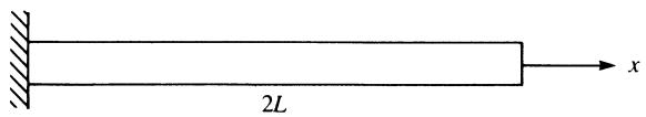# Example 16.3 For the bar shown in Figure 16–10 with length 2L, modulus of elasticity $E ,$ mass density $\rho ,$ and cross-sectional area A, determine the first two natural frequencies. 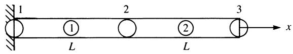For simplicity, the bar is discretized into two elements each of length L as shown in Figure 16–11. To solve Eq. (16.4.7), we must develop the total stiffness matrix for the bar by using Eq. (16.2.11). Either the lumped-mass matrix Eq. (16.2.12) or the 

text_image

2L x

Figure 16–10 One-dimensional bar used for natural frequency determination 

text_image

1 2 3 L L x

Figure 16–11 Discretized bar of Figure 16–10 consistent-mass matrix Eq. (16.2.23) can be used. In general, using the consistent-mass matrix has resulted in solutions that compare more closely to available analytical and experimental results than those found using the lumped-mass matrix. However, the longhand calculations are more tedious using the consistent-mass matrix than using the lumped-mass matrix because the consistent-mass matrix is a full symmetric matrix, whereas the lumped-mass matrix has nonzero terms only along the main diagonal. Hence, the lumped-mass matrix will be used in this analysis. Using Eq. (16.2.11), the stiffness matrices for each element are given by $$ [ \hat {k} ^ {(1)} ] = \frac {A E}{L} \left[ \begin{array}{c c} 1 & - 1 \\ - 1 & 1 \end{array} \right] \quad [ \hat {k} ^ {(2)} ] = \frac {A E}{L} \left[ \begin{array}{c c} 1 & - 1 \\ - 1 & 1 \end{array} \right] \tag {16.4.8} $$ The usual direct stiffness method for assembling the element matrices, Eqs. (16.4.8), yields the global stiffness matrix for the whole bar as $$ [ K ] = \frac {A E}{L} \left[ \begin{array}{r r r} 1 & - 1 & 0 \\ - 1 & 2 & - 1 \\ 0 & - 1 & 1 \end{array} \right] \tag {16.4.9} $$ Using Eq. (16.2.12), the mass matrices for each element are given by $$ [ \hat {m} ^ {(1)} ] = \frac {\rho A L}{2} \left[ \begin{array}{l l} 1 & 0 \\ 0 & 1 \end{array} \right] \quad [ \hat {m} ^ {(2)} ] = \frac {\rho A L}{2} \left[ \begin{array}{l l} 1 & 0 \\ 0 & 1 \end{array} \right] \tag {16.4.10} $$ The mass matrices for each element are assembled in the same manner as for the stiffness matrices. Therefore, by assembling Eqs. (16.4.10), we obtain the global mass matrix as $$ [ M ] = \frac {\rho A L}{2} \left[ \begin{array}{l l l} 1 & 0 & 0 \\ 0 & 2 & 0 \\ 0 & 0 & 1 \end{array} \right] \tag {16.4.11} $$ We observe from the resulting global mass matrix that there are two mass contributions at node 2 because node 2 is common to both elements. Substituting the global stiffness matrix Eq. (16.4.9) and the global mass matrix Eq. (16.4.11) into Eq. (16.4.6), and using the boundary condition $\hat { d } _ { 1 x } = 0$ (or now $d _ { 1 } ^ { \prime } = 0 )$ to reduce the set of equations in the usual manner, we obtain $$ \left(\frac {A E}{L} \left[ \begin{array}{c c} 2 & - 1 \\ - 1 & 1 \end{array} \right] - \omega^ {2} \frac {\rho A L}{2} \left[ \begin{array}{c c} 2 & 0 \\ 0 & 1 \end{array} \right]\right) \left\{ \begin{array}{l} d _ {2} ^ {\prime} \\ d _ {3} ^ {\prime} \end{array} \right\} = \left\{ \begin{array}{l} 0 \\ 0 \end{array} \right\} \tag {16.4.12} $$ To obtain a solution to the set of homogeneous equations in Eq. (16.4.12), we set the determinant of the coefficient matrix equal to zero as indicated by Eq. (16.4.7). We then have $$ \left| \frac {A E}{L} \left[ \begin{array}{c c} 2 & - 1 \\ - 1 & 1 \end{array} \right] - \lambda \frac {\rho A L}{2} \left[ \begin{array}{c c} 2 & 0 \\ 0 & 1 \end{array} \right] \right| = 0 \tag {16.4.13} $$ where $\lambda = \omega ^ { 2 }$ has been used in Eq. (16.4.13). Dividing Eq. (16.4.13) by $\rho A L$ and letting $\mu = E / ( \rho L ^ { 2 } )$ , we obtain $$ \left| \begin{array}{c c} 2 \mu - \lambda & - \mu \\ - \mu & \mu - \frac {\lambda}{2} \end{array} \right| = 0 \tag {16.4.14} $$ Evaluating the determinant in Eq. (16.4.14), we obtain $$ \lambda = 2 \mu \pm \mu \sqrt {2} $$ or $\lambda _ { 1 } = 0 . 6 0 \mu \qquad \lambda _ { 2 } = 3 . 4 1 \mu$ ð16:4:15Þ For comparison, the exact solution is given by $\lambda = 0 . 6 1 6 \mu$ , whereas the consistentmass approach yields $\lambda = 0 . 6 4 8 \mu$ . Therefore, for bar elements, the lumped-mass approach can yield results as good as, or even better than, the results for the consistent-mass approach. However, the consistent-mass approach can be mathematically proved to yield an upper bound on the frequencies, whereas the lumped-mass approach yields results that can be below or above the exact frequencies with no mathematical proof of boundedness. From Eqs. (16.4.15), the first and second natural frequencies are given by $$ \omega_ {1} = \sqrt {\lambda_ {1}} = 0. 7 7 \sqrt {\mu} \quad \omega_ {2} = \sqrt {\lambda_ {2}} = 1. 8 5 \sqrt {\mu} $$ Letting $E = 3 0 \times 1 0 ^ { 6 }$ psi, $\rho = 0 . 0 0 0 7 3 ~ \mathrm { { l b } } \mathrm { { - s } } ^ { 2 } / \mathrm { { i n } } ^ { 4 }$ , and $L = 1 0 0$ in., we obtain $$ \mu = E / (\rho L ^ {2}) = (3 0 \times 1 0 ^ {6}) / [ (0. 0 0 0 7 3) (1 0 0) ^ {2} ] = 4. 1 2 \times 1 0 ^ {6} \mathrm{s} ^ {- 2} $$ Therefore, we obtain the natural circular frequencies as $$ \omega_ {1} = 1. 5 6 \times 1 0 ^ {3} \mathrm{rad/s} \quad \omega_ {2} = 3. 7 6 \times 1 0 ^ {3} \mathrm{rad/s} \tag {16.4.16} $$ or in Hertz (1/s) units $$ f _ {1} = \omega_ {1} / 2 \pi = 2 4 8 \mathrm{Hz}, \quad \text { and so on } $$ In conclusion, note that for a bar discretized such that two nodes are free to displace, there are two natural modes and two frequencies. When a system vibrates with a given natural frequency $\omega _ { i } ,$ that unique shape with arbitrary amplitude corresponding to $\omega _ { i }$ is called the mode. In general, for an n-degrees-of-freedom discrete system, there are n natural modes and frequencies. A continuous system actually has an infinite number of natural modes and frequencies. When the system is discretized, only n degrees of freedom are created. The lowest modes and frequencies are approximated most often; the higher frequencies are damped out more rapidly and are usually of less importance. A rule of thumb is to use two times as many elements as the number of frequencies desired. 

area

| x | y | | ---- | ---- | | 0.7 | 0.7 | | 1.0 | 1.0 |

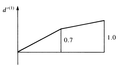
First mode 

line

| x | y | | ---- | ----- | | -0.7 | -0.7 | | 1.0 | 1.0 |

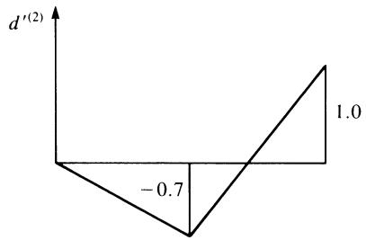
Second mode Figure 16–12 First and second modes of longitudinal vibration for the cantilever bar of Figure 16–10 Substituting $\lambda _ { 1 }$ from Eqs. (16.4.15) into Eq. (16.4.12) and simplifying, the first modal equations are given by $$ 1. 4 \mu d _ {2} ^ {\prime (1)} - \mu d _ {3} ^ {\prime (1)} = 0 $$ $$ - \mu d _ {2} ^ {\prime (1)} + 0. 7 \mu d _ {3} ^ {\prime (1)} = 0 \tag {16.4.17} $$ It is customary to specify the value of one of the natural modes $\underline { { d ^ { \prime } } }$ for a given $\omega _ { i }$ or $\lambda _ { i }$ . Letting $\check { d } _ { 3 } ^ { \prime ( 1 ) } = \mathsf { I }$ and solving Eq. (16.4.17), we find $d _ { 2 } ^ { \prime ( 1 ) } = 0 . 7$ . Similarly, substituting $\lambda _ { 2 }$ from Eqs. (16.4.15) into Eq. (16.4.12), we obtain the second modal equations. For brevity’s sake, these equations are not presented here. Now letting $d _ { 3 } ^ { \prime ( 2 ) } = 1$ results in $d _ { 2 } ^ { \prime ( 2 ) } = - 0 . 7$ . The modal response for the first and second natural frequencies of longitudinal vibration are plotted in Figure 16–12. The first mode means that the bar is completely in tension or compression, depending on the excitation direction. The second mode means the bar is in compression and tension or in tension and compression. 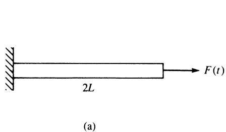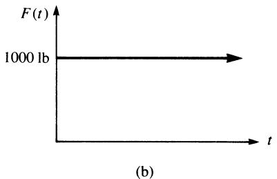# 16.5 Time-Dependent One-Dimensional Bar Analysis # Example 16.4 To illustrate the finite element solution of a time-dependent problem, we will solve the problem of the one-dimensional bar shown in Figure 16–13(a) subjected to the force shown in Figure 16–13(b). We will assume the boundary condition $d _ { 1 x } = 0$ and the initial conditions $\underline { { d } } _ { 0 } = 0$ and $\dot { \underline { d } } _ { 0 } = 0$ . For later numerical computation purposes, we let parameters $\rho = 0 . 0 0 0 7 3$ lb-s2/in4, A ¼ 1 in2, $E = 3 0 \times 1 0 ^ { 6 }$ psi, and $L = 1 0 0$ in. These parameters are the same values as used in Section 16.4. Because the bar is discretized into two elements of equal length, the global stiffness and mass matrices determined in Section 16.4 and given by Eqs. (16.4.9) and (16.4.11) are applicable. We will again use the lumped-mass matrix because of its 

text_image

2L (a) F(t)


text_image

F(t) 1000 lb (b)

Figure 16–13 (a) Bar subjected to a time-dependent force and (b) the forcing function applied to the end of the bar 

text_image

1 2 3 L L F(t)

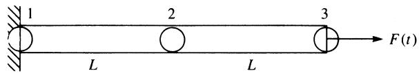
Figure 16–14 Discretized bar with lumped masses resulting computational simplicity. Figure 16–14 shows the discretized bar and the associated lumped masses. For illustration of the numerical time integration scheme, we will use the central difference method because it is easier to apply for longhand computations (and without loss of generality). We next select the time step to be used in the integration process. It has been mathematically shown that the time step must be less than or equal to 2 divided by the highest natural frequency when the central difference method is used [7]; that is, $\Delta t \leqslant 2 / \omega _ { \mathrm { m a x } }$ . However, for practical results, we must use a time step of less than or equal to three-fourths of this value; that is, $$ \Delta t \leqslant \frac {3}{4} \left(\frac {2}{\omega_ {\max}}\right) \tag {16.5.1} $$ This time step ensures stability of the integration method. This criterion for selecting a time step demonstrates the usefulness of determining the natural frequencies of vibration, as previously described in Section 16.4, before performing the dynamic stress analysis. An alternative guide (used only for a bar) for choosing the approximate time step is $$ \Delta t = \frac {L}{c _ {x}} \tag {16.5.2} $$ where L is the element length, and $c _ { x } = \sqrt { E _ { x } / \rho }$ is called the longitudinal wave velocity. Evaluating the time step by using both criteria, Eqs. (16.5.1) and (16.5.2), from Eqs. (16.4.16) for o, we obtain $$ \Delta t = \frac {3}{4} \left(\frac {2}{\omega_ {\max}}\right) = \frac {1 . 5}{3 . 7 6 \times 1 0 ^ {3}} = 0. 4 0 \times 1 0 ^ {- 3} \mathrm{s} \tag {16.5.3} $$ or $$ \Delta t = \frac {L}{c _ {x}} = \frac {1 0 0}{\sqrt {3 0 \times 1 0 ^ {6} / 0 . 0 0 0 7 3}} = 0. 4 8 \times 1 0 ^ {- 3} \mathrm{s} \tag {16.5.4} $$ Guided by the maximum time steps calculated in Eqs. (16.5.3) and (16.5.4), we choose $\Delta t = 0 . 2 5 \times 1 0 ^ { - 3 }$ s as a convenient time step for the computations. Substituting the global stiffness and mass matrices, Eqs. (16.4.9) and (16.4.11), into the global dynamic Eq. (16.2.24), we obtain $$ \frac {A E}{L} \left[ \begin{array}{r r r} 1 & - 1 & 0 \\ - 1 & 2 & - 1 \\ 0 & - 1 & 1 \end{array} \right] \left\{ \begin{array}{l} d _ {1 x} \\ d _ {2 x} \\ d _ {3 x} \end{array} \right\} + \frac {\rho A L}{2} \left[ \begin{array}{r r r} 1 & 0 & 0 \\ 0 & 2 & 0 \\ 0 & 0 & 1 \end{array} \right] \left\{ \begin{array}{l} \ddot {d} _ {1 x} \\ \ddot {d} _ {2 x} \\ \ddot {d} _ {3 x} \end{array} \right\} = \left\{ \begin{array}{l} R _ {1} \\ 0 \\ F _ {3} (t) \end{array} \right\} \tag {16.5.5} $$ where $R _ { 1 }$ denotes the unknown reaction at node 1. Using the procedure for solution outlined in Section 16.3 and in the flowchart of Figure 16–6, we begin as follows: # Step 1 Given: $d _ { 1 x } = 0$ because of the fixed support at node 1, and all nodal displacements and velocities are zero at time $t = 0 ;$ that is, $\dot { \underline { d } } _ { 0 } = 0$ and $\underline { { d } } _ { 0 } = 0$ . Also, assume $\ddot { d } _ { 1 x } = 0$ at all times. # Step 2 Solve for $\ddot { d } _ { 0 }$ using Eq. (16.3.5) as $$ \underline {{\ddot {d}}} _ {0} = \left\{ \begin{array}{l} \ddot {d} _ {2 x} \\ \ddot {d} _ {3 x} \end{array} \right\} _ {t = 0} = \frac {2}{\rho A L} \left[ \begin{array}{l l} \frac {1}{2} & 0 \\ 0 & 1 \end{array} \right] \left[ \left\{ \begin{array}{l} 0 \\ 1 0 0 0 \end{array} \right\} - \frac {A E}{L} \left[ \begin{array}{l l} 2 & - 1 \\ - 1 & 1 \end{array} \right] \left\{ \begin{array}{l} 0 \\ 0 \end{array} \right\} \right] \tag {16.5.6} $$ where Eq. (16.5.6) accounts for the conditions $d _ { 1 x } = 0$ and $\ddot { d } _ { 1 x } = 0$ . Simplifying Eq. (16.5.6), we obtain $$ \underline {{\ddot {d}}} _ {0} = \frac {2 0 0 0}{\rho A L} \left\{ \begin{array}{l} 0 \\ 1 \end{array} \right\} = \left\{ \begin{array}{c} 0 \\ 2 7, 4 0 0 \end{array} \right\} \text { in. } / \mathrm{s} ^ {2} \tag {16.5.7} $$ where the numerical values for $\rho , A ,$ , and L have been substituted into the final numerical result in Eq. (16.5.7), and $$ \underline {{M}} ^ {- 1} = \frac {2}{\rho A L} \left[ \begin{array}{l l} \frac {1}{2} & 0 \\ 0 & 1 \end{array} \right] \tag {16.5.8} $$ has been used in Eq. (16.5.6). The computational advantage of using the lumped-mass matrix for longhand calculations is now evident. The inverse of a diagonal matrix, such as the lumped-mass matrix, is obtained simply by inverting the diagonal elements of the matrix. # Step 3 Using Eq. (16.3.8), we solve for $\underline { d } _ { - 1 }$ as $$ \underline {{d}} _ {- 1} = \underline {{d}} _ {0} - (\Delta t) \underline {{\dot {d}}} _ {0} + \frac {(\Delta t) ^ {2}}{2} \ddot {\underline {{d}}} _ {0} \tag {16.5.9} $$ Substituting the initial conditions on $\dot{d}_{0}$ and $\dot{d}_{0}$ from step 1 and Eq. (16.5.7) for the initial acceleration $\dot{d}_{0}$ from step 2 into Eq. (16.5.9), we obtain $$ \underline {{d}} _ {- 1} = 0 - (0. 2 5 \times 1 0 ^ {- 3}) (0) + \frac {(0 . 2 5 \times 1 0 ^ {- 3}) ^ {2}}{2} (2 7, 4 0 0) \left\{ \begin{array}{l} 0 \\ 1 \end{array} \right\} $$ or, on simplification, $$ \left\{ \begin{array}{c} d _ {2 x} \\ d _ {3 x} \end{array} \right\} _ {- 1} = \left\{ \begin{array}{c} 0 \\ 0. 8 5 6 \times 1 0 ^ {- 3} \end{array} \right\} \text { in. } \tag {16.5.10} $$ # Step 4 On premultiplying Eq. (16.3.7) by $\underline{M}^{-1}$ , we now solve for $\underline{d}_1$ by $$ \underline {{d}} _ {1} = \underline {{M}} ^ {- 1} \{(\Delta t) ^ {2} \underline {{F}} _ {0} + [ 2 \underline {{M}} - (\Delta t) ^ {2} \underline {{K}} ] \underline {{d}} _ {0} - \underline {{M}} \underline {{d}} _ {- 1} \} \tag {16.5.11} $$ Substituting the numerical values for $\rho$ , A, L, and E and the results of Eq. (16.5.10) into Eq. (16.5.11), we obtain $$ \begin{array}{l} \left\{ \begin{array}{c} d _ {2 x} \\ d _ {3 x} \end{array} \right\} _ {1} = \frac {2}{0 . 0 7 3} \left[ \begin{array}{c c} \frac {1}{2} & 0 \\ 0 & 1 \end{array} \right] \left\{(0. 2 5 \times 1 0 ^ {- 3}) ^ {2} \left\{ \begin{array}{c} 0 \\ 1 0 0 0 \end{array} \right. \right\} + \left[ \frac {2 (0 . 0 7 3)}{2} \left[ \begin{array}{c c} 2 & 0 \\ 0 & 1 \end{array} \right] \right. \\ - (0. 2 5 \times 1 0 ^ {- 3}) ^ {2} (3 0 \times 1 0 ^ {4}) \left[ \begin{array}{c c} 2 & - 1 \\ - 1 & 1 \end{array} \right] \left\{ \begin{array}{l} 0 \\ 0 \end{array} \right\} \\ - \frac {0 . 0 7 3}{2} \left[ \begin{array}{c c} 2 & 0 \\ 0 & 1 \end{array} \right] \left\{ \begin{array}{c} 0 \\ 0. 8 5 6 \times 1 0 ^ {- 3} \end{array} \right\} \Bigg \} \\ \end{array} $$ Simplifying, we obtain $$ \left\{ \begin{array}{c} d _ {2 x} \\ d _ {3 x} \end{array} \right\} _ {1} = \frac {2}{0 . 0 7 3} \left[ \begin{array}{c c} \frac {1}{2} & 0 \\ 0 & 1 \end{array} \right] \left[ \left\{ \begin{array}{c} 0 \\ 0. 0 6 2 5 \times 1 0 ^ {- 3} \end{array} \right\} - \left\{ \begin{array}{c} 0 \\ 0. 0 3 1 2 \times 1 0 ^ {- 3} \end{array} \right\} \right] $$ Finally, the nodal displacements at time $t = 0.25 \times 10^{-3}$ s become $$ \left\{ \begin{array}{l} d _ {2 x} \\ d _ {3 x} \end{array} \right\} _ {1} = \left\{ \begin{array}{c} 0 \\ 0. 8 5 8 \times 1 0 ^ {- 3} \end{array} \right\} \text { in. } \quad \text {(at} t = 0. 2 5 \times 1 0 ^ {- 3} \text { s) } \tag {16.5.12} $$ # Step 5 With $\underline{d}_{0}$ initially given and $\underline{d}_{1}$ determined from step 4, we use Eq. (16.3.7) to obtain $$ \begin{array}{l} \underline {{d}} _ {2} = \underline {{M}} ^ {- 1} \{(\Delta t) ^ {2} \underline {{F}} _ {1} + [ 2 \underline {{M}} - (\Delta t) ^ {2} \underline {{K}} ] \underline {{d}} _ {1} - \underline {{M}} \underline {{d}} _ {0} \} \\ = \frac {2}{0 . 0 7 3} \left[ \begin{array}{c c} \frac {1}{2} & 0 \\ 0 & 1 \end{array} \right] \left\{(0. 2 5 \times 1 0 ^ {- 3}) ^ {2} \left\{ \begin{array}{c} 0 \\ 1 0 0 0 \end{array} \right\} + \left[ \frac {2 (0 . 0 7 3)}{2} \left[ \begin{array}{c c} 2 & 0 \\ 0 & 1 \end{array} \right] \right. \right. \\ - (0. 2 5 \times 1 0 ^ {- 3}) ^ {2} (3 0 \times 1 0 ^ {4}) \left[ \begin{array}{c c} 2 & - 1 \\ - 1 & 1 \end{array} \right] \Bigg ] \\ \end{array} $$