# Formulation An element’s formulation refers to the mathematical theory used to define the element’s behavior. In the Lagrangian, or material, description of behavior the element deforms with the material. In the alternative Eulerian, or spatial, description elements are fixed in space as the material flows through them. Eulerian methods are used commonly in fluid mechanics simulations. Abaqus/Standard uses Eulerian elements to model convective heat transfer. Abaqus/Explicit also offers multimaterial Eulerian elements for use in stress/displacement analyses. Adaptive meshing in Abaqus/Explicit combines the features of pure Lagrangian and Eulerian analyses and allows the motion of the element to be independent of the material (see “ALE adaptive meshing: overview,” Section 12.2.1). All other stress/displacement elements in Abaqus are based on the Lagrangian formulation. In Abaqus/Explicit the Eulerian elements can interact with Lagrangian elements through general contact (see “Eulerian analysis,” Section 14.1.1). To accommodate different types of behavior, some element families in Abaqus include elements with several different formulations. For example, the conventional shell element family has three classes: one suitable for general-purpose shell analysis, another for thin shells, and yet another for thick shells. In addition, Abaqus also offers continuum shell elements, which have nodal connectivities like continuum elements but are formulated to model shell behavior with as few as one element through the shell thickness. Some Abaqus/Standard element families have a standard formulation as well as some alternative formulations. Elements with alternative formulations are identified by an additional character at the end of the element name. For example, the continuum, beam, and truss element families include members with a hybrid formulation (to deal with incompressible or inextensible behavior); these elements are identified by the letter H at the end of the name (C3D8H or B31H). Abaqus/Standard uses the lumped mass formulation for low-order elements; Abaqus/Explicit uses the lumped mass formulation for all elements. As a consequence, the second mass moments of inertia can deviate from the theoretical values, especially for coarse meshes. In steady-state dynamic and frequency extraction procedures (see “Dynamic analysis procedures: overview,” Section 6.3.1), Abaqus/Standard uses a special projected mass matrix algorithm for the S3, S3R, S4, S4R, SC6R, SC8R, and S4R5 shell elements. As a consequence, slight differences may be observed in models that contain these elements when comparing results from steady-state dynamic and frequency extraction procedures to those of an implicit dynamic analysis. Abaqus/CFD uses hybrid elements to circumvent well known div-stability issues for incompressible flow. Abaqus/CFD also permits the addition of degrees of freedom based on procedure settings such as the optional energy equation and turbulence models. # Integration Abaqus uses numerical techniques to integrate various quantities over the volume of each element, thus allowing complete generality in material behavior. Using Gaussian quadrature for most elements, Abaqus evaluates the material response at each integration point in each element. Some continuum elements in Abaqus can use full or reduced integration, a choice that can have a significant effect on the accuracy of the element for a given problem. Abaqus uses the letter R at the end of the element name to label reduced-integration elements. For example, CAX4R is the 4-node, reduced-integration, axisymmetric, solid element. Shell, pipe, and beam element properties can be defined as general section behaviors; or each crosssection of the element can be integrated numerically, so that nonlinear response associated with nonlinear material behavior can be tracked accurately when needed. In addition, a composite layered section can be specified for shells and, in Abaqus/Standard, three-dimensional bricks, with different materials for each layer through the section. # Combining elements The element library is intended to provide a complete modeling capability for all geometries. Thus, any combination of elements can be used to make up the model; multi-point constraints (“General multi-point constraints,” Section 35.2.2) are sometimes helpful in applying the necessary kinematic relations to form the model (for example, to model part of a shell surface with solid elements and part with shell elements or to use a beam element as a shell stiffener). # Heat transfer and thermal-stress analysis In cases where heat transfer analysis is to be followed by thermal-stress analysis, corresponding heat transfer and stress elements are provided in Abaqus/Standard. See “Sequentially coupled thermal-stress analysis,” Section 16.1.2, for additional details. # Information available for element libraries The complete element library in Abaqus is subdivided into a number of smaller libraries. Each library is presented as a separate section in this guide. In each of these sections, information regarding the following topics is provided where applicable: • conventions; • element types; • degrees of freedom; • nodal coordinates required; • element property definition; • element faces; • element output; • nodes associated with the element; • loading (general loading, distributed loads, foundations, distributed heat fluxes, film conditions, radiation types, distributed flows, distributed impedances, electrical fluxes, distributed electric current densities, and distributed concentration fluxes); • node ordering and face ordering on elements; and • numbering of integration points for output. For element libraries that are available in both Abaqus/Standard and Abaqus/Explicit, individual element or load types that are available only in Abaqus/Standard are designated with an (S) ; similarly, individual element or load types that are available only in Abaqus/Explicit are designated with an (E) . Element or load types that are available in Abaqus/Aqua are designated with an (A) . Most of the element output variables available for an element are discussed. Additional variables may be available depending on the material model or the analysis procedure that is used. Some elements have solution variables that do not pertain to other elements of the same type; these variables are specified explicitly. # 27.1.2 CHOOSING THE ELEMENT’S DIMENSIONALITY Products: Abaqus/Standard Abaqus/Explicit Abaqus/CFD Abaqus/CAE # References • “Element library: overview,” Section 27.1.1 • “Part modeling space,” Section 11.4.1 of the Abaqus/CAE User’s Guide • “Assigning Abaqus element types,” Section 17.5 of the Abaqus/CAE User’s Guide # Overview The Abaqus element library contains the following for modeling a wide range of spatial dimensionality: • one-dimensional elements; • two-dimensional elements; • three-dimensional elements; • cylindrical elements; • axisymmetric elements; and • axisymmetric elements with nonlinear, asymmetric deformation. # One-dimensional (link) elements One-dimensional heat transfer, coupled thermal/electrical, and acoustic elements are available only in Abaqus/Standard. In addition, structural link (truss) elements are available in both Abaqus/Standard and Abaqus/Explicit. These elements can be used in two- or three-dimensional space to transmit loads or fluxes along the length of the element. # Two-dimensional elements Abaqus provides several different types of two-dimensional elements. For structural applications these include plane stress elements and plane strain elements. Abaqus/Standard also provides generalized plane strain elements for structural applications. # Plane stress elements Plane stress elements can be used when the thickness of a body or domain is small relative to its lateral (in-plane) dimensions. The stresses are functions of planar coordinates alone, and the out-of-plane normal and shear stresses are equal to zero. Plane stress elements must be defined in the X–Y plane, and all loading and deformation are also restricted to this plane. This modeling method generally applies to thin, flat bodies. For anisotropic materials the Z-axis must be a principal material direction. # Plane strain elements Plane strain elements can be used when it can be assumed that the strains in a loaded body or domain are functions of planar coordinates alone and the out-of-plane normal and shear strains are equal to zero. Plane strain elements must be defined in the X–Y plane, and all loading and deformation are also restricted to this plane. This modeling method is generally used for bodies that are very thick relative to their lateral dimensions, such as shafts, concrete dams, or walls. Plane strain theory might also apply to a typical slice of an underground tunnel that lies along the Z-axis. For anisotropic materials the Z-axis must be a principal material direction. Since plane strain theory assumes zero strain in the thickness direction, isotropic thermal expansion may cause large stresses in the thickness direction. 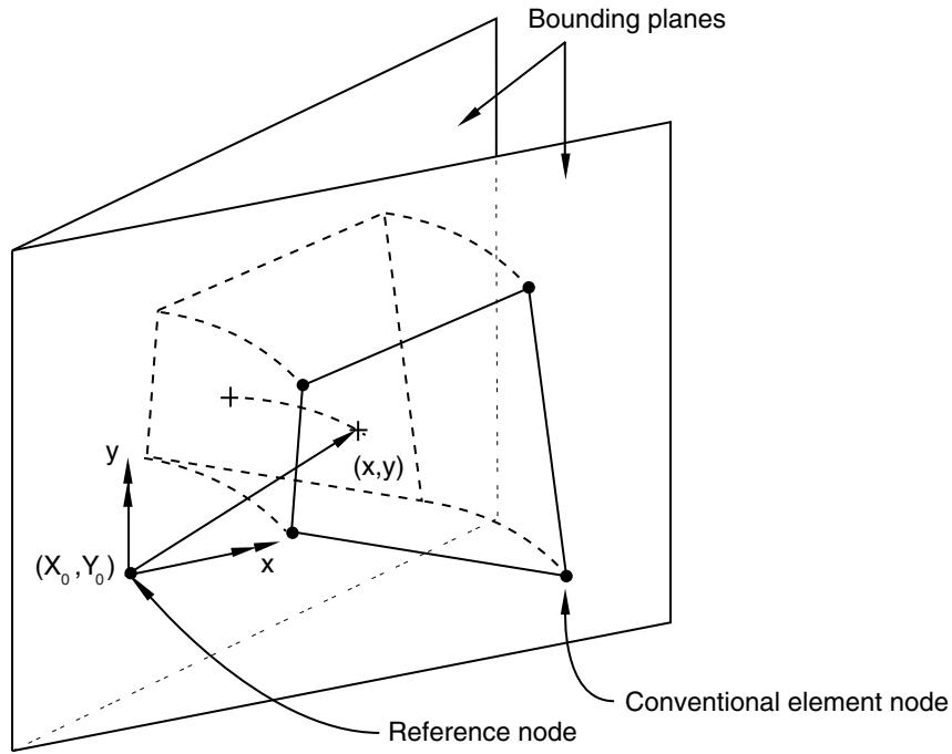# Generalized plane strain elements Generalized plane strain elements provide for the modeling of cases in Abaqus/Standard where the structure has constant curvature (and, hence, no gradients of solution variables) with respect to one material direction—the “axial” direction of the model. The formulation, thus, involves a model that lies between two planes that can move with respect to each other and, hence, cause strain in the axial direction of the model that varies linearly with respect to position in the planes, the variation being due to the change in curvature. In the initial configuration the bounding planes can be parallel or at an angle to each other, the latter case allowing the modeling of initial curvature of the model in the axial direction. The concept is illustrated in Figure 27.1.2–1. Generalized plane strain elements are typically used to model a section of a long structure that is free to expand axially or is subjected to axial loading. Each generalized plane strain element has three, four, six, or eight conventional nodes, at each of which x- and y-coordinates, displacements, etc. are stored. These nodes determine the position and motion of the element in the two bounding planes. Each element also has a reference node, which is usually the same node for all of the generalized plane strain elements in the model. The reference node of a generalized plane strain element should not be used as a conventional node in any element in the model. The reference node has three degrees of freedom 3, 4, and 5: $( \Delta u _ { z } , \Delta \phi _ { x }$ , and $\Delta \phi _ { y } )$ . The first degree of freedom $\left( \Delta u _ { z } \right)$ is the change in length of the axial material fiber connecting this node and its image in the other bounding plane. This displacement is positive as the planes move apart; therefore, there is a tensile strain in the axial fiber. The second and third degrees of freedom $( \Delta \phi _ { x } , \Delta \phi _ { y } )$ are the components of the relative rotation of one bounding plane with respect to the other. The values stored are the two components of rotation about the X- and Y-axes in the bounding planes (that is, in the cross-section of the model). Positive rotation about the X-axis causes increasing axial strain with respect to the y-coordinate in the cross-section; positive rotation about the Y-axis causes decreasing axial strain with respect to the x-coordinate in the cross-section. The x- and y-coordinates of a generalized plane strain element reference node $( X _ { 0 }$ and $Y _ { 0 }$ discussed below) remain fixed throughout all steps of an analysis. From the degrees of freedom of the reference node, the length of the axial material fiber passing through the point with current coordinates (x, y) in a bounding plane is defined as $$ t = t _ {0} + \Delta u _ {z} + (y - Y _ {0}) \Delta \phi_ {x} - (x - X _ {0}) \Delta \phi_ {y}, $$ 

text_image

Bounding planes (x,y) (x₀,Y₀) y x Reference node Conventional element node

Length of line through the thickness at $( \mathsf { x } , \mathsf { y } )$ is $$ t _ {0} + \Delta u _ {z} + \Delta \phi_ {x} (y - Y _ {0}) - \Delta \phi_ {y} (x - X _ {0}) $$ where quantities are defined in the text. Figure 27.1.2–1 Generalized plane strain model. where t $t _ { 0 }$ $\Delta u _ { z }$ $\Delta \phi _ { x }$ and $\Delta \phi _ { y }$ is the current length of the fiber, is the initial length of the fiber passing through the reference node (given as part of the element section definition), is the displacement at the reference node (stored as degree of freedom 3 at the reference node), are the total values of the components of the angle between the bounding planes (the original values of $\Delta \phi _ { x } , \ \Delta \phi _ { y }$ are given as part of the element section definition—see “Defining the element’s section properties” in “Solid (continuum) elements,” Section 28.1.1: the changes in these values are the degrees of freedom 4 and 5 of the reference node), and $X _ { 0 }$ and $Y _ { 0 }$ are the coordinates of the reference node in a bounding plane. The strain in the axial direction is defined immediately from this axial fiber length. The strain components in the cross-section of the model are computed from the displacements of the regular nodes of the elements in the usual way. Since the solution is assumed to be independent of the axial position, there are no transverse shear strains. # Three-dimensional elements Three-dimensional elements are defined in the global X, Y, Z space. These elements are used when the geometry and/or the applied loading are too complex for any other element type with fewer spatial dimensions. # Cylindrical elements Cylindrical elements are three-dimensional elements defined in the global X, Y, Z space. These elements are used to model bodies with circular or axisymmetric geometry subjected to general, nonaxisymmetric loading. Cylindrical elements are available only in Abaqus/Standard. Cylindrical elements are useful in situations where the expected solution over a relatively large angle is nearly axisymmetric. In this case a very coarse mesh of cylindrical elements is often sufficient. Footprint and steady-state rolling analyses of tires are good examples of where cylindrical elements have distinct advantages over conventional continuum elements (see “Steady-state rolling analysis of a tire,” Section 3.1.2 of the Abaqus Example Problems Guide). If, however, the expected solution has significant non-axisymmetric components, a finer mesh of cylindrical elements will be needed and it may be more economical to use conventional continuum elements. 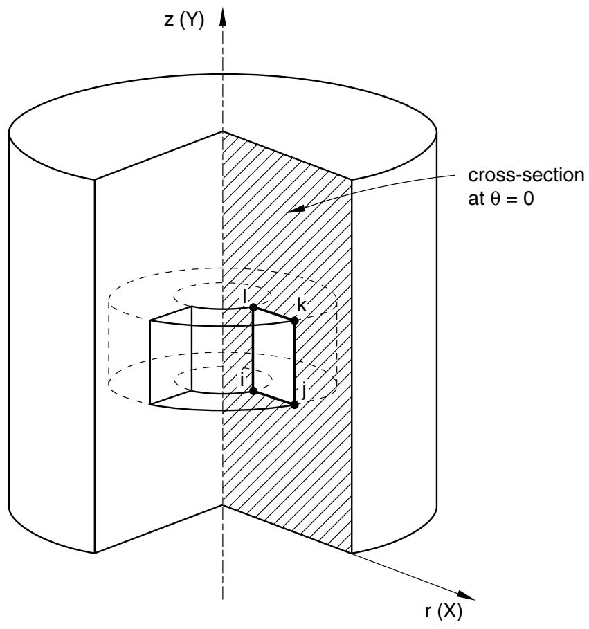# Axisymmetric elements Axisymmetric elements provide for the modeling of bodies of revolution under axially symmetric loading conditions. A body of revolution is generated by revolving a plane cross-section about an axis (the symmetry axis) and is readily described in cylindrical polar coordinates r, z, and . Figure 27.1.2–2 shows a typical reference cross-section at $\theta = 0$ . The radial and axial coordinates of a point on this cross-section are denoted by r and z, respectively. At , the radial and axial coordinates coincide with the global Cartesian X- and Y-coordinates. Abaqus does not apply boundary conditions automatically to nodes that are located on the symmetry axis in axisymmetric models. If required, you should apply them directly. Radial boundary conditions at nodes located on the z-axis are appropriate for most problems because without them nodes may displace across the symmetry axis, violating the principle of compatibility. However, there are some analyses, such as penetration calculations, where nodes along the symmetry axis should be free to move; boundary conditions should be omitted in these cases. If the loading and material properties are independent of , the solution in any r–z plane completely defines the solution in the body. Consequently, axisymmetric elements can be used to analyze the 

text_image

z (Y) cross-section at θ = 0 l k i j r (X)

Figure 27.1.2–2 Reference cross-section and element in an axisymmetric solid. problem by discretizing the reference cross-section at $\theta = 0$ . Figure 27.1.2–2 shows an element of an axisymmetric body. The nodes $i , j , k ,$ and l are actually nodal “circles,” and the volume of material associated with the element is that of a body of revolution, as shown in the figure. The value of a prescribed nodal load or reaction force is the total value on the ring; that is, the value integrated around the circumference. # Regular axisymmetric elements Regular axisymmetric elements for structural applications allow for only radial and axial loading and have isotropic or orthotropic material properties, with being a principal direction. Any radial displacement in such an element will induce a strain in the circumferential direction (“hoop” strain); and since the displacement must also be purely axisymmetric, there are only four possible nonzero components of strain $( \varepsilon _ { r r } , \varepsilon _ { z z } , \varepsilon _ { \theta \theta } , \mathrm { a n d } \gamma _ { r z } )$ . 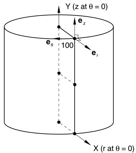# Generalized axisymmetric stress/displacement elements with twist Axisymmetric solid elements with twist are available only in Abaqus/Standard for the analysis of structures that are axially symmetric but can twist about their symmetry axis. This element family is similar to the axisymmetric elements discussed above, except that it allows for a circumferential loading component (which is independent of ) and for general material anisotropy. Under these conditions, there may be displacements in the -direction that vary with r and z but not with . The problem remains axisymmetric because the solution does not vary as a function of so that the deformation of any r–z plane characterizes the deformation in the entire body. Initially the elements define an axisymmetric reference geometry with respect to the r–z plane at $\theta \ : = \ : 0$ , where the r-direction corresponds to the global X-direction and the z-direction corresponds to the global Y-direction. Figure 27.1.2–3 shows an axisymmetric model consisting of two elements. The figure also shows the local cylindrical coordinate system at node 100. 

text_image

Y (z at θ = 0) e_z e_θ 100 e_r X (r at θ = 0)

(a) 

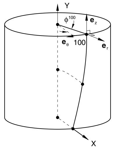
text_image

Y φ100 eθ 100 e_z e_r X

(b) Figure 27.1.2–3 Reference and deformed cross-section in an axisymmetric solid with twist. The motion at a node of an axisymmetric element with twist is described by the radial displacement $u _ { r } ,$ , the axial displacement $u _ { z }$ , and the twist $\phi$ (in radians) about the z-axis, each of which is constant in the circumferential direction, so that the deformed geometry remains axisymmetric. Figure 27.1.2–3(b) shows the deformed geometry of the reference model shown in Figure 27.1.2–3(a) and the local cylindrical coordinate system at the displaced location of node 100, for a twist $\phi ^ { 1 0 0 }$ . The formulation of these elements is discussed in “Axisymmetric elements,” Section 3.2.8 of the Abaqus Theory Guide.