# 31.2.9 CONNECTOR FAILURE BEHAVIOR Products: Abaqus/Standard Abaqus/Explicit Abaqus/CAE # References • “Connectors: overview,” Section 31.1.1 • “Connector behavior,” Section 31.2.1 • \*CONNECTOR BEHAVIOR • \*CONNECTOR FAILURE • “Defining failure,” Section 15.17.11 of the Abaqus/CAE User’s Guide, in the HTML version of this guide # Overview Connector failure behavior: • can be defined in any connector with available components of relative motion in Abaqus/Standard; • can be defined in any connector in Abaqus/Explicit; • can be used in Abaqus/Standard to fail all or specified components of relative motion if a failure criterion is met; • can be used in Abaqus/Explicit to fail all or specified components if a failure criterion is met; • can be triggered if either a connector relative motion or connector force in a specified component is outside a specified range; and • can be replaced in most cases by the more sophisticated connector damage initiation/evolution behavior (see “Connector damage behavior,” Section 31.2.7). # Defining connector failure behavior A typical connector might have pieces that break if a relative motion component, force, or moment becomes too large. Abaqus provides a way to define which components of relative motion will break and the criteria used to release these components. You can select the component of relative motion on which the failure criterion is based. In Abaqus/Standard connector failure can be used to specify connector behavior based on available components of relative motion. In Abaqus/Explicit connector failure can be used to specify connector behavior based on constrained as well as available components of relative motion. Limit values for force or moment can be specified for all components of relative motion involved in the connection. In addition, for connectors with available components of relative motion, limit values can be specified for the relative positions corresponding to an available component. In Abaqus/Standard if the failure criterion specified for the selected component of relative motion is met, either all components of relative motion fail or a single available component fails. By default, all components of relative motion are released upon meeting the failure criterion. The nodal force contributions for all released components from the connector element will be removed during the increment when the failure criterion is met. In Abaqus/Explicit if the failure criterion specified for the selected component is met, either all components or a single available component fails. By default, all components are released upon meeting the failure criterion. The nodal force contributions for all released components from the connector element will be removed during the increment when the failure criterion is met. Input File Usage: Use the following options to define connector failure: \*CONNECTOR BEHAVIOR, NAME=name \*CONNECTOR FAILURE, COMPONENT=component number, RELEASE=ALL or component number Abaqus/CAE Usage: Interaction module: connector section editor: Add→Failure: Components: component or components, Release: All or Specify component # Viscous damping in Abaqus/Standard In Abaqus/Standard the sudden release of the failed connection may lead to convergence problems. To avoid convergence problems, you can add viscous damping to the components. Damping forces in the component are calculated as $F _ { i } ~ = ~ \mu v _ { i }$ , where $\mu$ is the user-defined damping coefficient and $v _ { i }$ is the velocity of the failed component. Viscous damping is applied only if a selected available component of relative motion is released. Input File Usage: Use the following options to add viscous damping to failed components in Abaqus/Standard: \*SECTION CONTROLS, NAME=name, VISCOSITY= $* { \mathrm { C O N N E C T O R ~ S E C T I O N } } , { \mathrm { C O N T R O L S } } { = } { n a m e }$ Abaqus/CAE Usage: Viscous regularization is not supported in Abaqus/CAE. 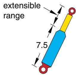# Example In the example in Figure 31.2.9–1 assume that the shock absorber pulls apart if the tensile force in the shock exceeds 800.0 units of force. 

text_image

extensible range 7.5


text_image

node 12 b 1 (local orientation) a node 11 2

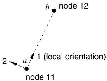
Figure 31.2.9–1 Simplified connector model of a shock absorber. ```txt ... *CONNECTOR BEHAVIOR, NAME=sbehavior *CONNECTOR FAILURE, COMPONENT=1, RELEASE=ALL , , , 800.0 ``` # Output The Abaqus output variables available for connectors are listed in “Abaqus/Standard output variable identifiers,” Section 4.2.1, and “Abaqus/Explicit output variable identifiers,” Section 4.2.2. The following output variables are of particular interest when defining failure in connectors: CFAILST Flags for connector failure status. ALLVD Energy dissipated by viscous damping added to failed components. At any given time and for a particular component of relative motion i, the output variable CFAILSTi is 1 if the connector fails in that particular component of relative motion (failure criteria are met). If the failure criteria are not met at a given time for a particular component i, the output variable CFAILSTi is 0. # 31.2.10 CONNECTOR UNIAXIAL BEHAVIOR # Product: Abaqus/Explicit # References • “Connectors: overview,” Section 31.1.1 • “Connector behavior,” Section 31.2.1 • \*CONNECTOR BEHAVIOR • \*LOADING DATA • \*UNLOADING DATA # Overview Connector uniaxial behavior: • can be defined in any connector with available components of relative motion by specifying the loading and unloading behavior; • can be specified for each available component of relative motion independently; • can define separate response in the tensile and compressive directions; • can exhibit nonlinear elastic behavior, damaged elastic behavior, or elastic-plastic type behavior with permanent deformation upon complete unloading; • can have an unloading response specified; and • can be specified as dependent on constitutive motions in several local directions. The local directions for each connection type (as described in “Connection-type library,” Section 31.1.5) determine the directions in which the forces and moments act and in which the displacements and rotations are measured. # Specifying uniaxial behavior for an available component of relative motion Uniaxial behavior can be specified for an available component of relative motion by defining the loading and unloading response for that component. For each component, separate loading/unloading response data can be defined for the response in the tensile and compressive directions. The loading and unloading response can be classified according to three available behavior types: • nonlinear elastic behavior; • damaged elastic behavior; and • elastic-plastic type behavior with permanent deformation. To define the loading response, you specify forces or moments as nonlinear functions of the components of relative motion. These functions can also depend on temperature, field variables, and constitutive displacements/rotations in the other component directions. See “Input syntax rules,” Section 1.2.1, for further information about defining data as functions of temperature and field variables. The unloading response can be defined in the following ways: • You can specify several unloading curves that express the forces or moments as nonlinear functions of the components of relative motion; Abaqus interpolates these curves to create an unloading curve that passes through the point of unloading in an analysis. • You can specify an energy dissipation factor (and a permanent deformation factor for models with permanent deformation), from which Abaqus calculates an exponential/quadratic unloading function. • You can specify the forces or moments as nonlinear functions of the components of relative motion, as well as a transition slope; the connector unloads along the specified transition slope until it intersects the specified unloading function, at which point it unloads according to the function. (This unloading definition is referred to as combined unloading.) • You can specify the forces or moments as nonlinear functions of the components of relative motion; Abaqus shifts the specified unloading function along the strain axis so that it passes through the point of unloading in an analysis. The behavior type that is specified for the loading response dictates the type of unloading you can define, as summarized in Table 31.2.10–1. The different behavior types, as well as the associated loading and unloading curves, are discussed in more detail in the sections that follow. Table 31.2.10–1 Available unloading definitions for the uniaxial behavior types.

Material behavior type	Unloading definition
	Interpolated	Quadratic	Exponential	Combined	Shifted
Rate-dependent elastic	√
Damaged elastic	√	√	√	√
Permanent deformation	√	√	√		√

# Input File Usage: Use the following options to define connector uniaxial behavior: \*CONNECTOR BEHAVIOR, NAME=name \*CONNECTOR UNIAXIAL BEHAVIOR, COMPONENT=component number \*LOADING DATA, DIRECTION=deformation direction, TYPE=behavior type data lines to define loading data \*UNLOADING DATA data lines to define unloading data # Defining the deformation direction The loading/unloading data can be defined separately for tension and compression by specifying the deformation direction. If the deformation direction is defined (tension or compression), the tabular values defining tensile or compressive behavior should be specified with positive values of forces/moments and displacements/rotations in the specified component of relative motion and the loading data must start at the origin. If the behavior is not defined in a loading direction, the force response will be zero in that direction (the connector has no resistance in that direction). If the deformation direction is not defined, the data apply to both tension and compression. However, the behavior is then considered to be nonlinear elastic and no damage or permanent deformation can be specified. The response data will be considered to be symmetric about the origin if either tensile or compressive data are omitted. Input File Usage: Use the following option to define tensile behavior: \*LOADING DATA, DIRECTION=TENSION Use the following option to define compressive behavior: \*LOADING DATA, DIRECTION=COMPRESSION Use the following option to define both tensile compressive behavior in a single table: \*LOADING DATA # Behavior that depends on relative positions or motions in multiple component directions By default, the loading and unloading functions depend only on the displacement or rotation in the direction of the component of relative motion specified for the connector uniaxial behavior definition (see “Connector behavior,” Section 31.2.1, for details). However, it is also possible to define loading and unloading functions that depend on the constitutive displacements and rotations in multiple component directions. 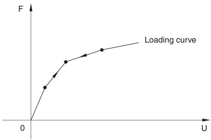Input File Usage: Use the following option to define connector uniaxial behavior that depends on the relative displacements and/or rotations in several component directions: \*LOADING DATA, INDEPENDENT COMPONENTS=CONSTITUTIVE MOTION # Defining rate-independent nonlinear elastic behavior When the loading response is rate independent, the unloading response is also rate independent and occurs along the same user-specified loading curve as illustrated in Figure 31.2.10–1. An unloading curve does not need to be specified. 

line

| U | F | | ---- | ----- | | 0 | 0 | | >0 | Increasing |

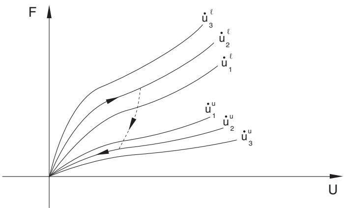
Figure 31.2.10–1 Nonlinear elastic loading. Input File Usage: \*LOADING DATA, TYPE=ELASTIC # Defining rate-dependent behavior The rate-dependent models require the specification of force-displacement curves at different rates of deformation to describe both loading and unloading behavior. If unloading behavior is not specified, the unloading occurs along the loading curve with the smallest rate of deformation. As the rate of deformation changes, the response is obtained by interpolation of the specified loading/unloading data. Unphysical jumps in the forces due to sudden changes in the rate of deformation are prevented using a technique based on viscoplastic regularization. This technique also helps model relaxation effects in a very simplistic manner, with the relaxation time given as $\tau = \mu _ { 0 } + \mu _ { 1 } | \lambda - 1 | ^ { \alpha }$ , where $\mu _ { 0 } , \mu _ { 1 }$ , and are material parameters and is the stretch. $\mu _ { 0 }$ is a linear viscosity parameter that controls the relaxation time when $\lambda \approx 1$ . Small values of this parameter should be used. $\mu _ { 1 }$ is a nonlinear viscosity parameter that controls the relaxation time at higher values of . The smaller this value, the shorter the relaxation time. controls the sensitivity of the relaxation speed to the stretch in the component of relative motion. Suggested values of these parameters are $\mu _ { 0 } = 0 . 0 0 0 1 , \mu _ { 1 } = 0 . 0 0 5$ , and $\alpha = 2$ . Figure 31.2.10–2 illustrates the loading/unloading behavior as the connector is loaded at a rate $\dot { u } _ { 2 } ^ { l }$ and then unloaded at a rate ${ \dot { u } _ { 2 } } ^ { u }$ . 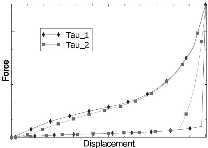Figure 31.2.10–3 shows the loading/unloading response of a connector element for two different relaxation times $\tau _ { 1 }$ and $\tau _ { 2 }$ with $\tau _ { 2 } > \tau _ { 1 }$ . The larger the relaxation time, the longer it takes to achieve the specified loading/unloading response for the applied deformation rate. 

line

| U | u̇₁ | u̇₂ | u̇₃ | u̇₃ | u̇₃ | |-------|---------|---------|---------|---------|---------| | 0 | 0 | 0 | 0 | 0 | 0 | | 1 | ~0.5 | ~0.7 | ~0.9 | ~1.1 | ~1.3 | | 2 | ~1.0 | ~1.3 | ~1.6 | ~1.9 | ~2.2 | | 3 | ~1.5 | ~1.9 | ~2.2 | ~2.5 | ~2.8 |

Figure 31.2.10–2 Rate-dependent loading/unloading. 

line

| Displacement | Tau_1 | Tau_2 | | ------------ | ----- | ----- | | 0 | 0 | 0 | | 1 | 0.5 | 0.3 | | 2 | 1.0 | 0.6 | | 3 | 1.5 | 0.9 | | 4 | 2.0 | 1.2 | | 5 | 2.5 | 1.5 | | 6 | 3.0 | 1.8 | | 7 | 3.5 | 2.1 | | 8 | 4.0 | 2.4 | | 9 | 4.5 | 2.7 | | 10 | 5.0 | 3.0 | | 11 | 5.5 | 3.3 | | 12 | 6.0 | 3.6 | | 13 | 6.5 | 3.9 | | 14 | 7.0 | 4.2 | | 15 | 7.5 | 4.5 | | 16 | 8.0 | 4.8 | | 17 | 8.5 | 5.1 | | 18 | 9.0 | 5.4 | | 19 | 9.5 | 5.7 | | 20 | 10.0 | 6.0 | | 21 | 10.5 | 6.3 | | 22 | 11.0 | 6.6 | | 23 | 11.5 | 6.9 | | 24 | 12.0 | 7.2 | | 25 | 12.5 | 7.5 | | 26 | 13.0 | 7.8 | | 27 | 13.5 | 8.1 | | 28 | 14.0 | 8.4 | | 29 | 14.5 | 8.7 | | 30 | 15.0 | 9.0 | | 31 | 15.5 | 9.3 | | 32 | 16.0 | 9.6 | | 33 | 16.5 | 9.9 | | 34 | 17.0 | 10.2 | | 35 | 17.5 | 10.5 | | 36 | 18.0 | 10.8 | | 37 | 18.5 | 11.1 | | 38 | 19.0 | 11.4 | | 39 | 19.5 | 11.7 | | 40 | 20.0 | 12.0 | | 41 | 20.5 | 12.3 | | 42 | 21.0 | 12.6 | | 43 | 21.5 | 12.9 | | 44 | 22.0 | 13.2 | | 45 | 22.5 | 13.5 | | 46 | 23.0 | 13.8 | | 47 | 23.5 | 14.1 | | 48 | 24.0 | 14.4 | | 49 | 24.5 | 14.7 | | 50 | 25.0 | 15.0 | | 51 | 25.5 | 15.3 | | 52 | 26.0 | 15.6 | | 53 | 26.5 | 15.9 | | 54 | 27.0 | 16.2 | | 55 | 27.5 | 16.5 | | 56 | 28.0 | 16.8 | | 57 | 28.5 | 17.1 | | 58 | 29.0 | 17.4 | | 59 | 29.5 | 17.7 | | 60 | 30.0 | 18.0 | | 61 | 30.5 | 18.3 | | 62 | 31.0 | 18.6 | | 63 | 31.5 | 18.9 | | 64 | 32.0 | 19.2 | | 65 | 32.5 | 19.5 | | 66 | 33.0 | 19.8 | | 67 | 33.5 | 20.1 | | 68 | 34.0 | 20.4 | | 69 | 34.5 | 20.7 | | 70 | 35.0 | 21.0 | | 71 | 35.5 | 21.3 | | 72 | 36.0 | 21.6 | | 73 | 36.5 | 21.9 | | 74 | 37.0 | 22.2 | | 75 | 37.5 | 22.5 | | 76 | 38.0 | 22.8 | | 77 | 38.5 | 23.1 | | 78 | 39.0 | 23.4 | | 79 | 39.5 | 23.7 | | 80 | 40.0 | 24.0 | | 81 | 40.5 | 24.3 | | 82 | 41.0 | 24.6 | | 83 | 41.5 | 24.9 | | 84 | 42.0 | 25.2 | | 85 | 42.5 | 25.5 | | 86 | 43.0 | 25.8 | | 87 | 43.5 | 26.1 | | 88 | 44.0 | 26.4 | | 89 | 44.5 | 26.7 | | 90 | 45.0 | 27.0 | | 91 | 45.5 | 27.3 | | 92 | 46.0 | 27.6 | | 93 | 46.5 | 27.9 | | 94 | 47.0 | 28.2 | | 95 | 47.5 | 28.5 | | 96 | 48.0 | 28.8 | | 97 | 48.5 | 29.1 | | 98 | 49.0 | 29.4 | | 99 | 49.5 | 29.7 | | 100 | 50.0 | 30.0 |

Figure 31.2.10–3 Rate-dependent loading/unloading. # Input File Usage: Use the following options when the unloading is also rate dependent: \*LOADING DATA, TYPE=ELASTIC, RATE DEPENDENT \*UNLOADING DATA, DEFINITION=INTERPOLATED CURVE, RATE DEPENDENT Use the following options when the unloading is rate independent: \*LOADING DATA, TYPE=ELASTIC, RATE DEPENDENT \*UNLOADING DATA, DEFINITION=INTERPOLATED CURVE # Defining models with damage The damage models dissipate energy upon unloading, and there is no permanent deformation upon complete unloading. The unloading behavior controls the amount of energy dissipated by damage mechanisms and can be specified in one of the following ways: • an analytical unloading curve (exponential/quadratic); • an unloading curve interpolated from multiple user-specified unloading curves; or • unloading along a transition unloading curve (constant slope specified by user) to the user-specified unloading curve (combined unloading). For an overview of the different available behaviors, see “Specifying uniaxial behavior for an available component of relative motion” above. The various unloading types are discussed in the sections that follow. # Defining onset of damage You can specify the onset of damage by defining the displacement below which unloading occurs along the loading curve. Input File Usage: \*LOADING DATA, TYPE=DAMAGE, DAMAGE ONSET=value # Specifying exponential/quadratic unloading The damage model in Figure 31.2.10–4 is based on an analytical unloading curve that is derived from an energy dissipation factor, (fraction of energy that is dissipated at any displacement level). As the connector is loaded, the force follows the path given by the loading curve. If the connector is unloaded (for example, at point B), the force follows the unloading curve . Reloading after unloading follows the unloading curve until the loading is such that the displacement becomes greater than , after which the loading path follows the loading curve. The arrows shown in Figure 31.2.10–4 illustrate the loading/unloading paths of this model. The unloading response follows the loading curve when the calculated unloading curve lies above the loading curve to prevent energy generation and follows a zero force response when the unloading curve yields a negative response. In such cases the dissipated energy will be less than the value specified by the energy dissipation factor. Input File Usage: Use the following option to define quadratic unloading behavior: \*UNLOADING DATA, DEFINITION=QUADRATIC Use the following option to define exponential unloading behavior: \*UNLOADING DATA, DEFINITION=EXPONENTIAL # Specifying interpolated curve unloading The damage model in Figure 31.2.10–5 illustrates an interpolated unloading response based on multiple unloading curves that intersect the primary loading curve at increasing values of forces/displacements. You can specify as many unloading curves as are necessary to define the unloading response. Each