# Defining contact blockage in Abaqus/Explicit In Abaqus/Explicit you can control the combination of surfaces that can cause blockage of flow out of a surface-based fluid cavity. The details of contact blockage are discussed in “Contact blockage,” Section 37.1.4. # Defining a friction model By default, Abaqus assumes that contact between surfaces is frictionless. You can include a friction model as part of a surface interaction definition. Details of the various friction models available in Abaqus are discussed in “Frictional behavior,” Section 37.1.5. # User-defined interfacial constitutive behavior Instead of choosing one or some combination of the various interfacial behavior models that are available in Abaqus, you can define any special or proprietary interfacial constitutive behavior through a user subroutine. In Abaqus/Standard you can use the subroutine UINTER; whereas in Abaqus/Explicit you can use VUINTER if you are using the contact pair algorithm and VUINTERACTION if you are using the general contact algorithm. In Abaqus/Explicit a penalty enforcement of the contact constraint must be used for interacting surfaces whose interfacial behavior is governed by VUINTER or VUINTERACTION. Details of the definition of a user-defined interfacial constitutive behavior are discussed in “Userdefined interfacial constitutive behavior,” Section 37.1.6. # Defining a pressure penetration load in Abaqus/Standard You can define pressure penetration loads to simulate the penetration of fluid between two contacting surfaces in Abaqus/Standard. The details of the pressure penetration model are discussed in “Pressure penetration loading,” Section 37.1.7. # Defining the interaction of debonded surfaces in Abaqus/Standard You can allow two initially bonded surfaces to debond in Abaqus/Standard, as discussed in “Crack propagation analysis,” Section 11.4.3. The details of the contact interaction model after debonding are discussed in “Interaction of debonded surfaces,” Section 37.1.8. # Defining breakable bonds in Abaqus/Explicit In Abaqus/Explicit you can define breakable bonds that connect the interacting surfaces. The kinematic contact pair algorithm must be used when defining breakable bonds. The breakable bonds affect both the relative tangential motion and the motion normal to the surfaces. Breakable bonds cannot be used with analytical rigid surfaces. The details of the breakable bond model, known as the spot weld model, are discussed in “Breakable bonds,” Section 37.1.9. # Defining surface-based cohesive behavior You can define surface-based cohesive behavior to model delamination of initially bonded surfaces or to model “sticky” contact between parts that are initially separated but bond on coming into contact, with the possibility that the bond may undergo progressive damage and fail. Surface-based cohesive behavior is modeled within the general contact framework in Abaqus/Explicit and within the contact pair framework in Abaqus/Standard. The details of the surface-based cohesive behavior model are discussed in “Surface-based cohesive behavior,” Section 37.1.10. # 37.1.2 CONTACT PRESSURE-OVERCLOSURE RELATIONSHIPS Products: Abaqus/Standard Abaqus/Explicit Abaqus/CAE # References • “Mechanical contact properties: overview,” Section 37.1.1 • \*CONTACT CONTROLS • \*SURFACE BEHAVIOR • “Creating interaction properties,” Section 15.12.2 of the Abaqus/CAE User’s Guide, in the HTML version of this guide • “Customizing contact controls,” Section 15.12.3 of the Abaqus/CAE User’s Guide, in the HTML version of this guide # Overview In Abaqus the following contact pressure-overclosure relationships can be used to define the contact model: • the “hard” contact relationship minimizes the penetration of the slave surface into the master surface at the constraint locations and does not allow the transfer of tensile stress across the interface; • a “softened” contact relationship in which the contact pressure is a linear function of the clearance between the surfaces; • a “softened” contact relationship in which the contact pressure is an exponential function of the clearance between the surfaces (in Abaqus/Explicit this relationship is available only for the contact pair algorithm); • a “softened” contact relationship in which a tabular pressure-overclosure curve is constructed by progressively scaling the default penalty stiffness (available only for general contact in Abaqus/Explicit); • a “softened” contact relationship in which the contact pressure is a piecewise linear (tabular) function of the clearance between the surfaces; and • a relationship in which there is no separation of the surfaces once they contact. In addition, a viscous damping relationship can be defined that will affect the pressure-overclosure relationship; see “Contact damping,” Section 37.1.3, for more information. In Abaqus/Standard pressure penetration loads can be applied to model fluid penetrating into the surface between two contacting bodies; see “Pressure penetration loading,” Section 37.1.7. # Including a contact pressure-overclosure relationship in a contact property definition By default, a “hard” contact pressure-overclosure relationship is used for both surface-based contact and element-based contact. You can include a nondefault contact pressure-overclosure relationship in a specific contact property definition. Input File Usage: Use both of the following options for surface-based contact: \*SURFACE INTERACTION, NAME=interaction\_property\_name \*SURFACE BEHAVIOR Use both of the following options for element-based contact in Abaqus/Standard: \*INTERFACE or \*GAP, ELSET=name \*SURFACE BEHAVIOR Abaqus/CAE Usage: Interaction module: contact property editor: Mechanical→Normal Behavior: Constraint enforcement method: Default Element-based contact is not supported in Abaqus/CAE. # Using the “hard” contact relationship The most common contact pressure-overclosure relationship is shown in Figure 37.1.2–1, although the zero-penetration condition may or may not be strictly enforced depending on the constraint enforcement method used (the constraint enforcement methods are discussed in “Contact constraint enforcement methods in Abaqus/Standard,” Section 38.1.2, and “Contact constraint enforcement methods in Abaqus/Explicit,” Section 38.2.3). When surfaces are in contact, any contact pressure can be transmitted between them. The surfaces separate if the contact pressure reduces to zero. Separated surfaces come into contact when the clearance between them reduces to zero. Input File Usage: \*SURFACE BEHAVIOR (omit the PRESSURE-OVERCLOSURE parameter to obtain the default “hard” pressure-overclosure relationship) Abaqus/CAE Usage: Interaction module: contact property editor: Mechanical→Normal Behavior: Constraint enforcement method: Default: Pressure-Overclosure: Hard Contact # Considerations for rigid-to-rigid contact in Abaqus/Explicit For general contact in Abaqus/Explicit involving two rigid bodies with complete displacement control loading, the contact forces may be noisy due to effects of the number of contact interactions involving each rigid body and the contact penalty stiffness. This same effect will not occur with force control loading. The solution of the analysis should still remain stable. 

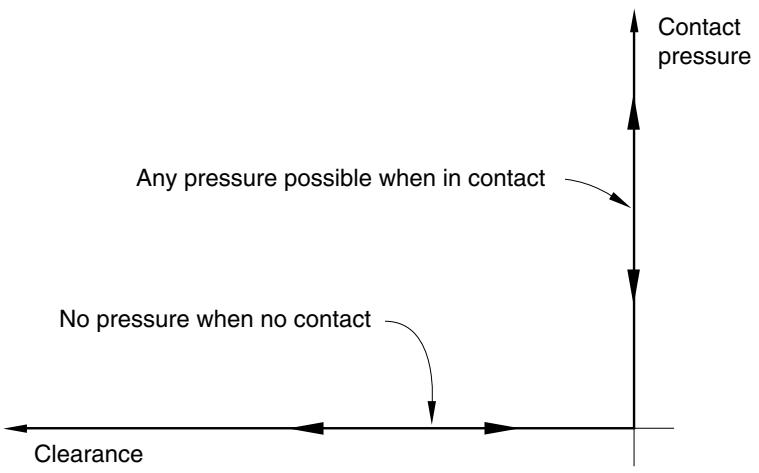
text_image

Contact pressure Any pressure possible when in contact No pressure when no contact Clearance

Figure 37.1.2–1 Default pressure-overclosure relationship. # Using a “softened” contact relationship Three types of “softened” contact relationships are available in Abaqus. The pressure-overclosure relationship can be prescribed by using a linear law, a tabular piecewise-linear law, or an exponential law (in Abaqus/Explicit available only with the contact pair algorithm). For contact involving element-based surfaces and for element-based contact (available only in Abaqus/Standard), the “softened” contact relationships are specified in terms of overclosure (or clearance) versus contact pressure. For contact involving a node-based surface or nodal contact elements (such as GAP and ITT elements) for which an area or length dimension is not defined, softened contact is specified in terms of overclosure (or clearance) versus contact force. For slave surfaces on beam-type elements in Abaqus/Standard and for the contact pair algorithm in Abaqus/Explicit, specify pressure as force per unit length. If the general contact algorithm in Abaqus/Explicit is being used for slave surfaces on beam-type elements, specify pressure as force per unit area. When using softened contact relationships that have nonzero pressure at zero overclosure (not allowed with the general contact algorithm) in Abaqus/Explicit, you should be aware that initial, nonequilibrated contact pressures may be present in the analysis (see “Adjusting initial surface positions and specifying initial clearances for contact pairs in Abaqus/Explicit,” Section 36.5.4). # “Softened” contact versus “hard” contact The “softened” contact pressure-overclosure relationships might be used to model a soft, thin layer on one or both surfaces. In Abaqus/Standard they are also sometimes useful for numerical reasons because they can make it easier to resolve the contact condition. # Using “softened” contact in implicit dynamic simulations Use the softened contact relationship with caution in implicit dynamic impact simulations. If this relationship is used in such a simulation, Abaqus/Standard will not use the impact algorithm, which destroys kinetic energy of the nodes on the surface when impact occurs, but will instead assume a perfectly elastic collision. The consequence of this change is that the slave nodes bounce back immediately after impact with the master surface; hence, extensive “chattering” may result, leading to convergence problems and small time increments. However, softened contact may work well in implicit dynamic calculations where impact effects are not important; for example, if contact changes are primarily due to sliding motion along a curved surface, such as may occur in low-speed metal forming applications. # Using “softened” contact in explicit dynamic simulations In Abaqus/Explicit softened contact can be enforced with either the kinematic or the penalty constraint enforcement method (see “Contact constraint enforcement methods in Abaqus/Explicit,” Section 38.2.3, for details). With penalty enforcement the contact collisions are elastic except for the influence of contact damping, whereas with softened kinematic contact some energy will be absorbed by the impact because of algorithmic characteristics: the energy absorbed tends to increase as the contact stiffness increases. Another consideration is the effect on the time increment: with kinematic enforcement the stable time increment is independent of the contact stiffness, but with penalty contact the time increment decreases as the contact stiffness increases. # “Softened” contact defined as a linear function In a linear pressure-overclosure relationship the surfaces transmit contact pressure when the overclosure between them, measured in the contact (normal) direction, is greater than zero. The linear pressureoverclosure relationship is identical to a tabular relationship with two data points, where the first point is located at the origin. You specify the slope of the pressure-overclosure relationship, k. 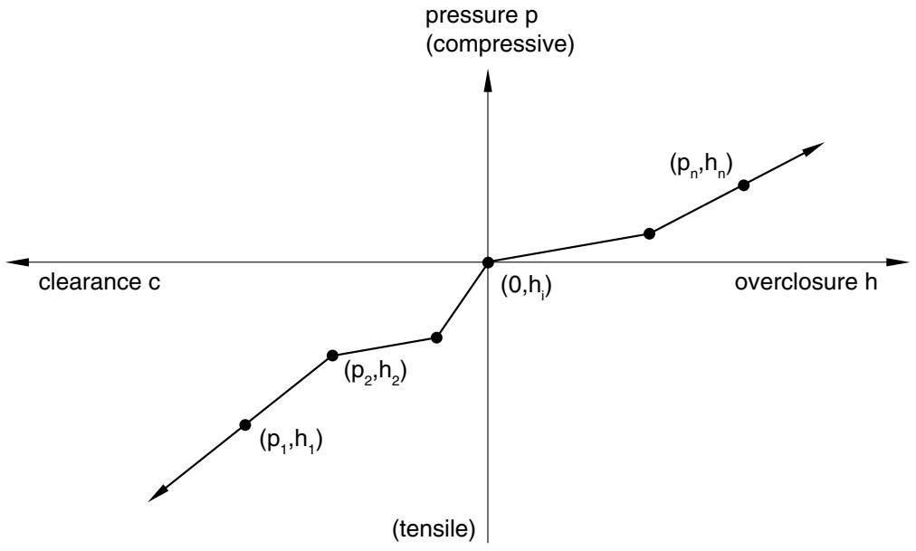Input File Usage: \*SURFACE BEHAVIOR, PRESSURE-OVERCLOSURE=LINEAR k Abaqus/CAE Usage: Interaction module: contact property editor: Mechanical→Normal Behavior: Constraint enforcement method: Default: Pressure-Overclosure: Linear, Contact stiffness: k # “Softened” contact defined in tabular form To define a piecewise-linear pressure-overclosure relationship in tabular form, as shown in Figure 37.1.2–2, you specify data pairs $( p _ { i } , \ h _ { i } )$ of pressure versus overclosure (where overclosure corresponds to negative clearance). You must specify the data as an increasing function of pressure and overclosure. In this relationship the surfaces transmit contact pressure when the overclosure between them, measured in the contact (normal) direction, is greater than $h _ { 1 }$ , where $h _ { 1 }$ is the overclosure at zero pressure. For the general contact algorithm in Abaqus/Explicit $h _ { 1 }$ must be zero. For overclosures greater than $h _ { n }$ the pressure-overclosure relationship is extrapolated based on the last slope computed from the user-specified data (see Figure 37.1.2–2). 

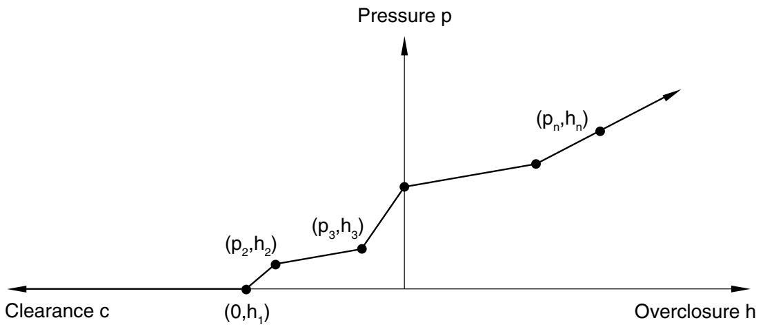
line

| Overclosure h | Pressure p | Label | | ------------- | ---------- | --------- | | 0 | (0,h₁) | (p₂,h₂) | | 0 | (p₃,h₃) | (p₃,h₃) | | 0 | (pₙ,hₙ) | (pₙ,hₙ) |

Figure 37.1.2–2 “Softened” pressure-overclosure relationship defined in tabular form. Input File Usage: \*SURFACE BEHAVIOR, PRESSURE-OVERCLOSURE=TABULAR Abaqus/CAE Usage: Interaction module: contact property editor: Mechanical→Normal Behavior: Constraint enforcement method: Default: Pressure-Overclosure: Tabular # “Softened” contact defined as a geometric scaling of the default contact stiffness An alternative piecewise linear tabular pressure-overclosure relationship can be constructed by geometrically scaling the default contact stiffness. This model provides a simple interface to increase the default contact stiffness when a critical penetration is exceeded. A penetration measure, $d ,$ i s defined either directly or as a fraction, , of the minimum element length, $L _ { e l e m : }$ , in the contact region. Each time the current penetration exceeds a multiple of this penetration measure, the contact stiffness is scaled by a factor, (see Figure 37.1.2–3). The initial stiffness is set equal to the default contact stiffness, $k _ { d f l t }$ , multiplied by a factor, $s _ { 0 }$ . This option is available only for the general contact algorithm in Abaqus/Explicit. Input File Usage: \*SURFACE BEHAVIOR, PRESSURE-OVERCLOSURE=SCALE FACTOR Abaqus/CAE Usage: Interaction module: contact property editor: Mechanical→Normal Behavior: Constraint enforcement method: Default: Pressure-Overclosure: Scale Factor (General Contact) 

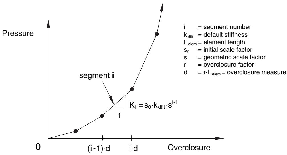
line

| Overclosure | Pressure | | ----------- | -------- | | 0 | 0 | | (i-1)·d | 1 | | i·d | K_i = s_0 · k_dflt · s^{i-1} | | >i·d | >1 |

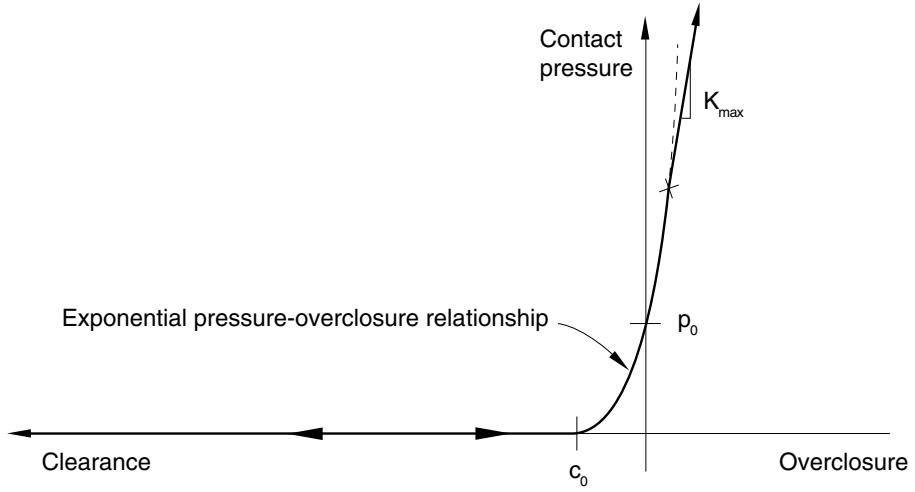
Figure 37.1.2–3 “Softened” scale factor pressure-overclosure relationship. # “Softened” contact defined with an exponential law In an exponential (soft) contact pressure-overclosure relationship the surfaces begin to transmit contact pressure once the clearance between them, measured in the contact (normal) direction, reduces to $c _ { 0 }$ . The contact pressure transmitted between the surfaces then increases exponentially as the clearance continues to diminish. Figure 37.1.2–4 illustrates this behavior in Abaqus/Standard. In Abaqus/Explicit this behavior is available only for the contact pair algorithm. In Abaqus/Explicit you can specify an optional limit on the contact stiffness that the model can attain, $k _ { m a x }$ (see Figure 37.1.2–5); this limit is useful for penalty contact to mitigate the effect that large stiffnesses have on reducing the stable time increment. By default, $k _ { m a x }$ will be set to infinity for kinematic contact and to the default penalty stiffness for penalty contact. You specify $c _ { 0 } ;$ ; the contact pressure at zero clearance, $p _ { 0 } ;$ and, optionally in Abaqus/Explicit, $k _ { m a x } .$ Input File Usage: $* { \mathrm { S U R F A C E ~ B E H A V I O R } } , { \mathrm { P R E S S U R E - O V E R C L O S U R E = E X P O N E N T I A L } }$ $c _ { 0 } , p _ { 0 } , k _ { m a x }$ Abaqus/CAE Usage: Interaction module: contact property editor: Mechanical→Normal Behavior: Constraint enforcement method: Default: Pressure-Overclosure: Exponential, Pressure $p _ { 0 }$ , Clearance $c _ { 0 }$ , Specify: $k _ { m a x }$ # Using the no separation relationship You can indicate that Abaqus should use the contact pressure-overclosure relationship that prevents surfaces from separating once they have come into contact. In Abaqus/Explicit this relationship can 

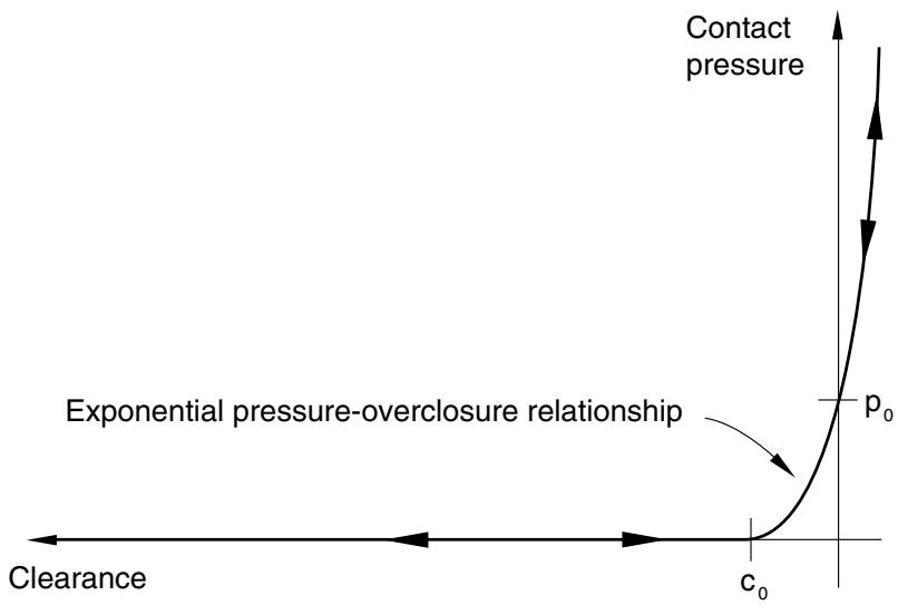
text_image

Contact pressure Exponential pressure-overclosure relationship p₀ c₀ Clearance

Figure 37.1.2–4 Exponential “softened” pressure-overclosure relationship in Abaqus/Standard. 

text_image

Contact pressure Kmax Exponential pressure-overclosure relationship p0 Clearance c0 Overclosure

Figure 37.1.2–5 Exponential “softened” pressure-overclosure relationship in Abaqus/Explicit. be specified for general contact but only for pure master-slave contact pairs, and it cannot be used with adaptive meshing. The no separation relationship is often used with the rough friction model (see “Frictional behavior,” Section 37.1.5) to model nonintermittent, rough frictional contact. Using this combination of surface interaction models causes surfaces to remain fully bonded together (no separation and no tangential sliding) once they contact, even if the contact pressure between them is tensile. Input File Usage: \*SURFACE BEHAVIOR, NO SEPARATION Abaqus/CAE Usage: Interaction module: contact property editor: Mechanical→Normal Behavior: Constraint enforcement method: Default: Pressure-Overclosure: Hard, toggle off Allow separation after contact # “Softened” contact with the no separation relationship in Abaqus/Explicit In Abaqus/Explicit if a softened contact relationship is specified with the no separation relationship, the pressure-overclosure relationship will include tensile behavior. The exponential relationship cannot be used with no separation behavior. For the tabular relationship, a point must be specified on the zero pressure axis, and the slope will continue into the tensile regime following the same slope as the first two data points (see Figure 37.1.2–6). The linear relationship will have a linear tensile pressure-overclosure relationship with the same slope that is used for the compressive behavior. 

line

| Point Label | Overclosures | Pressure (p) | |-------------|-------------|--------------| | (p₁,h₁) | 0 | (0,hᵢ) | | (p₂,h₂) | 0 | (0,hᵢ) | | (pₙ,hₙ) | 0 | (0,hᵢ) |

Figure 37.1.2–6 Piecewise linear “softened” pressure-overclosure relationship with tensile behavior in Abaqus/Explicit. # Surface interaction output variables related to the contact pressure-overclosure Abaqus/Standard provides both the clearance, COPEN, and the contact pressure, CPRESS, as output to the data, results, and output database files. Output to these files is requested as described in “Output to the data and results files,” Section 4.1.2, and “Output to the output database,” Section 4.1.3.