text_image

I₃ 6R ④ ② 2R ③ 4R I₁ 2R ① B 2E A E I₂

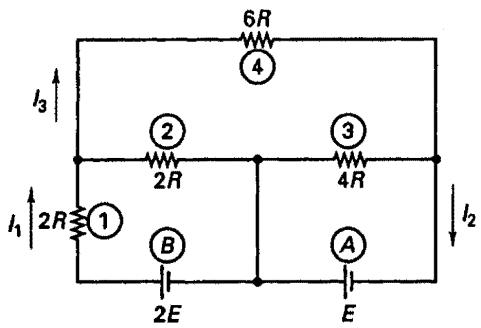
Figure E3.4 Dc network Writing these equations in matrix form, we obtain $$ \left[ \begin{array}{c c c} 4 R & 0 & - 2 R \\ 0 & 4 R & - 4 R \\ - 2 R & - 4 R & 1 2 R \end{array} \right] \left[ \begin{array}{l} I _ {1} \\ I _ {2} \\ I _ {3} \end{array} \right] = \left[ \begin{array}{c} 2 E \\ E \\ 0 \end{array} \right] \tag {a} $$ The analysis is completed by solving these equations for $I_{1}$ , $I_{2}$ , and $I_{3}$ . Note that the equilibrium equations in (a) could also have been established using a direct stiffness procedure, as in Examples 3.1 to 3.3. We should note once again that the steps of analysis in the preceding structural, heat transfer, fluid flow, and electrical problems are very similar, the basic analogy being possibly best expressed in the use of the direct stiffness procedure for each problem. This indicates that the same basic numerical procedures will be applicable in the analysis of almost any physical problem (see Chapters 4 and 7). Each of these examples deals with a linear system; i.e., the coefficient matrix is constant and thus, if the right-hand-side forcing functions are multiplied by a constant $\alpha$ , the system response is also $\alpha$ times as large. We consider in this chapter primarily linear systems, but the same steps for solution summarized previously are also applicable in nonlinear analysis, as demonstrated in the following example (see also Chapters 6 and 7). 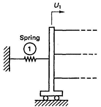EXAMPLE 3.5: Consider the spring-cart system in Fig. E3.1 and assume that spring ① now has the nonlinear behavior shown in Fig. E3.5. Discuss how the equilibrium equations given in Example 3.1 have to be modified for this analysis. 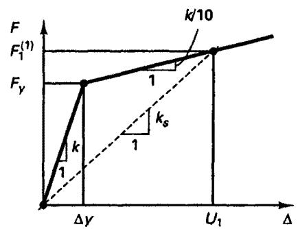As long as $U_{1} \leq \Delta y$ , the equilibrium equations in Example 3.1 are applicable with $k_{1} = k$ . However, if the loads are such that $U_{1} > \Delta y$ , i.e., $F_{1}^{(1)} > F_{y}$ , we need to use a different value for $k_{1}$ , and this value depends on the force $F_{1}^{(1)}$ acting in the element. Denoting the stiffness value by $k_{s}$ , as shown in Fig. E3.5, the response of the system is described for any load by the equilibrium equations $$ \mathbf {K} _ {s} \mathbf {U} = \mathbf {R} \tag {a} $$ where the coefficient matrix is established exactly as in Example 3.1 but using $k_{s}$ instead of $k_{1}$ , $$ \mathbf {K} _ {s} = \left[ \begin{array}{c c c} \left(k _ {s} + k _ {2} + k _ {3} + k _ {4}\right) & - \left(k _ {2} + k _ {3}\right) & - k _ {4} \\ - \left(k _ {2} + k _ {3}\right) & \left(k _ {2} + k _ {3} + k _ {5}\right) & - k _ {5} \\ - k _ {4} & - k _ {5} & \left(k _ {4} + k _ {5}\right) \end{array} \right] \tag {b} $$ 

text_image

Spring 1 U₁


line

| Δy | Fy | k/10 | |------|------|------| | Δy | Fy | k | | U1 | Fy | k |

Figure E3.5 Spring ① of the cart-spring system of Fig. E3.1 with nonlinear elastic characteristics Although the response of the system can be calculated using this approach, in which $K_{s}$ is referred to as the secant matrix, we will see in Chapter 6 that in general practical analysis we actually use an incremental procedure with a tangent stiffness matrix. These analyses demonstrate the general analysis procedure: the selection of unknown state variables that characterize the response of the system under consideration, the identification of elements that together comprise the complete system, the establishment of the element equilibrium requirements, and finally the assemblage of the elements by invoking interelement continuity requirements. A few observations should be made. First, we need to recognize that there is some choice in the selection of the state variables. For example, in the analysis of the carts in Example 3.1, we could have chosen the unknown forces in the springs as state variables. A second observation is that the equations from which the state variables are calculated can be linear or nonlinear equations and the coefficient matrix can be of a general nature. However, it is most desirable to deal with a symmetric positive definite coefficient matrix because in such cases the solution of the equations is numerically very effective (see Section 8.2). In general, the physical characteristics of a problem determine whether the numerical solution can actually be cast in a form that leads to a symmetric positive definite coefficient matrix. However, even if possible, a positive definite coefficient matrix is obtained only if appropriate solution variables are selected, and in a nonlinear analysis an appropriate linearization must be performed in the iterative solution. For this reason, in practice, it is valuable to employ general formulations for whole classes of problems (e.g., structural analysis, heat transfer, and so on—see Sections 4.2, 7.2, and 7.3) that for any analysis lead to a symmetric and positive definite coefficient matrix. In the preceding discussion we employed the direct approach of assembling the system-governing equilibrium equations. An important point is that the governing equilibrium equations for state variables can in many analyses also be obtained using an extremum, or variational formulation. An extremum problem consists of locating the set (or sets) of values (state variables) $U_{i}, i = 1, \ldots, n$ , for which a given functional $\Pi(U_{i}, \ldots, U_{n})$ is a maximum, is a minimum, or has a saddle point. The condition for obtaining the equations for the state variables is $$ \delta \Pi = 0 \tag {3.1} $$ and since $\delta \Pi = \frac{\partial\Pi}{\partial U_1}\delta U_1 + \dots +\frac{\partial\Pi}{\partial U_n}\delta U_n$ (3.2) we must have $\frac{\partial\Pi}{\partial U_i} = 0$ for $i = 1,\dots ,n$ (3.3) We note that $\delta U_{i}$ stands for “variations in the state variables $U_{i}$ that are arbitrary except that they must be zero at and corresponding to the state variable boundary conditions.” $^{1}$ The second derivatives of $\Pi$ with respect to the state variables then decide whether the solution corresponds to a maximum, a minimum, or a saddle point. In the solution of lumped-parameter models we can consider that $\Pi$ is defined such that the relations in (3.3) generate the governing equilibrium equations. $^{2}$ For example, in linear structural analysis, when displacements are used as state variables, $\Pi$ is the total potential (or total potential energy) $$ \Pi = \mathcal {U} - \mathcal {W} \tag {3.4} $$ where U is the strain energy of the system and W is the total potential of the loads. The solution for the state variables corresponds in this case to the minimum of $\Pi$ . EXAMPLE 3.6: Consider a simple spring of stiffness k and applied load P, and discuss the use of (3.1) and (3.4). Let u be the displacement of the spring under the load P. We then have $$ \mathcal {U} = \frac {1}{2} k u ^ {2}; \quad \mathcal {W} = P u $$ and $\Pi = \frac{1}{2} ku^2 - Pu$ Note that for a given $P$ , we could graph $\Pi$ as a function of $u$ . Using (3.1) we have, with $u$ as the only variable, $$ \delta \Pi = (k u - P) \delta u; \quad \frac {\partial \Pi}{\partial u} = k u - P $$ which gives the equilibrium equation $$ k u = P \tag {a} $$ Using (a) to evaluate $\mathcal{W}$ , we have at equilibrium $\mathcal{W} = ku^2$ ; i.e., $\mathcal{W} = 2^{\mathfrak{Q}}l$ and $\Pi = -\frac{1}{2}ku^2 = -\frac{1}{2}Pu$ . Also, $\partial^2\Pi/\partial u^2 = k$ and hence at equilibrium $\Pi$ is at its minimum. EXAMPLE 3.7: Consider the analysis of the system of rigid carts in Example 3.1. Determine $\Pi$ and invoke the condition in (3.1) for obtaining the governing equilibrium equations. Using the notation defined in Example 3.1, we have $$ \mathcal {U} = \frac {1}{2} \mathbf {U} ^ {T} \mathbf {K} \mathbf {U} \tag {a} $$ and $\mathcal{W} = \mathbf{U}^T\mathbf{R}$ (b) where it should be noted that the total strain energy in (a) could also be written as $$ \begin{array}{l} \mathcal {U} = \frac {1}{2} \mathbf {U} ^ {T} \left(\sum_ {i = 1} ^ {5} \mathbf {K} ^ {(i)}\right) \mathbf {U} \\ = \frac {1}{2} \mathbf {U} ^ {T} \mathbf {K} ^ {(1)} \mathbf {U} + \frac {1}{2} \mathbf {U} ^ {T} \mathbf {K} ^ {(2)} \mathbf {U} + \dots + \frac {1}{2} \mathbf {U} ^ {T} \mathbf {K} ^ {(5)} \mathbf {U} \\ = \mathfrak {U} _ {1} + \mathfrak {U} _ {2} + \dots + \mathfrak {U} _ {5} \\ \end{array} $$ where $\mathcal{U}_i$ is the strain energy stored in the $i$ th element. Using (a) and (b), we now obtain $$ \boldsymbol {\Pi} = \frac {1}{2} \mathbf {U} ^ {T} \mathbf {K} \mathbf {U} - \mathbf {U} ^ {T} \mathbf {R} \tag {c} $$ Applying (3.1) gives $$ \mathbf {K U} = \mathbf {R} $$ Solving for U and then substituting into (c), we find that $\Pi$ corresponding to the displacements at system equilibrium is $$ \Pi = - \frac {1}{2} \mathbf {U} ^ {T} \mathbf {R} $$ Since the same equilibrium equations are generated using the direct solution approach and the variational approach, we may ask what the advantages of employing a variational scheme are. Assume that for the problem under consideration $\Pi$ is defined. The equilibrium equations can then be generated by simply adding the contributions from all elements to $\Pi$ and invoking the stationarity condition in (3.1). In essence, this condition generates automatically the element interconnectivity requirements. Thus, the variational technique can be very effective because the system-governing equilibrium equations can be generated “quite mechanically.” The advantages of a variational approach are even more pronounced when we consider the numerical solution of a continuous system (see Section 3.3.2). However, a main disadvantage of a variational approach is that, in general, less physical insight into a problem formulation is obtained than when using the direct approach. Therefore, it may be critical that we interpret physically the system equilibrium equations, once they have been established using a variational approach, in order to identify possible errors in the solution and in order to gain a better understanding of the physical meaning of the equations. # 3.2.2 Propagation Problems The main characteristic of a propagation or dynamic problem is that the response of the system under consideration changes with time. For the analysis of a system, in principle, the same procedures as in the analysis of a steady-state problem are employed, but now the state variables and element equilibrium relations depend on time. The objective of the analysis is to calculate the state variables for all time t. Before discussing actual propagation problems, let us consider the case where the time effect on the element equilibrium relations is negligible but the load vector is a function of time. In this case the system response is obtained using the equations governing the steady-state response but substituting the time-dependent load or forcing vector for the load vector employed in the steady-state analysis. Since such an analysis is in essence still a steady-state analysis, but with steady-state conditions considered at any time t, the analysis may be referred to as a pseudo steady-state analysis. In an actual propagation problem, the element equilibrium relations are time-dependent, and this accounts for major differences in the response characteristics when compared to steady-state problems. In the following we present two examples that demonstrate the formulation of the governing equilibrium equations in propagation problems. Methods for calculating the solution of these equations are given in Chapter 9. EXAMPLE 3.8: Consider the system of rigid carts that was analyzed in Example 3.1. Assume that the loads are time-dependent and establish the equations that govern the dynamic response of the system. For the analysis we assume that the springs are massless and that the carts have masses $m_{1}$ , $m_{2}$ , and $m_{3}$ (which amounts to lumping the distributed mass of each spring to its two end points). Then, using the information given in Example 3.1 and invoking d'Alembert's principle, the element interconnectivity requirements yield the equations $$ F _ {1} ^ {(1)} + F _ {1} ^ {(2)} + F _ {1} ^ {(3)} + F _ {1} ^ {(4)} = R _ {1} (t) - m _ {1} \ddot {U} _ {1} $$ $$ F _ {2} ^ {(2)} + F _ {2} ^ {(3)} + F _ {2} ^ {(5)} = R _ {2} (t) - m _ {2} \ddot {U} _ {2} $$ $$ F _ {3} ^ {(4)} + F _ {3} ^ {(5)} = R _ {3} (t) - m _ {3} \ddot {U} _ {3} $$ where $\ddot{U}_i = \frac{d^2U_i}{dt^2};\qquad i = 1,2,3$ Thus we obtain as the system-governing equilibrium equations $$ \mathbf {M} \ddot {\mathbf {U}} + \mathbf {K} \mathbf {U} = \mathbf {R} (t) \tag {a} $$ where K, U, and R have been defined in Example 3.1 and M is the system mass matrix $$ \mathbf {M} = \left[ \begin{array}{c c c} m _ {1} & 0 & 0 \\ 0 & m _ {2} & 0 \\ 0 & 0 & m _ {3} \end{array} \right] $$ The equilibrium equations in (a) represent a system of ordinary differential equations of second order in time. For the solution of these equations it is also necessary that the initial conditions on U and $\dot{U}$ be given; i.e., we need to have ${}^{0}U$ and ${}^{0}\dot{U}$ , where $$ { } ^ { 0 } \mathbf { U } = \mathbf { U } | _ { t = 0 } ; \quad { } ^ { 0 } \dot { \mathbf { U } } = \dot { \mathbf { U } } | _ { t = 0 } $$ Earlier we mentioned the case of a pseudo steady-state analysis. Considering the response of the carts, such analysis implies that the loads change very slowly and hence mass effects can be neglected. Therefore, to obtain the pseudo steady-state response, the equilibrium equations (a) in Example 3.8 should be solved with M = 0. 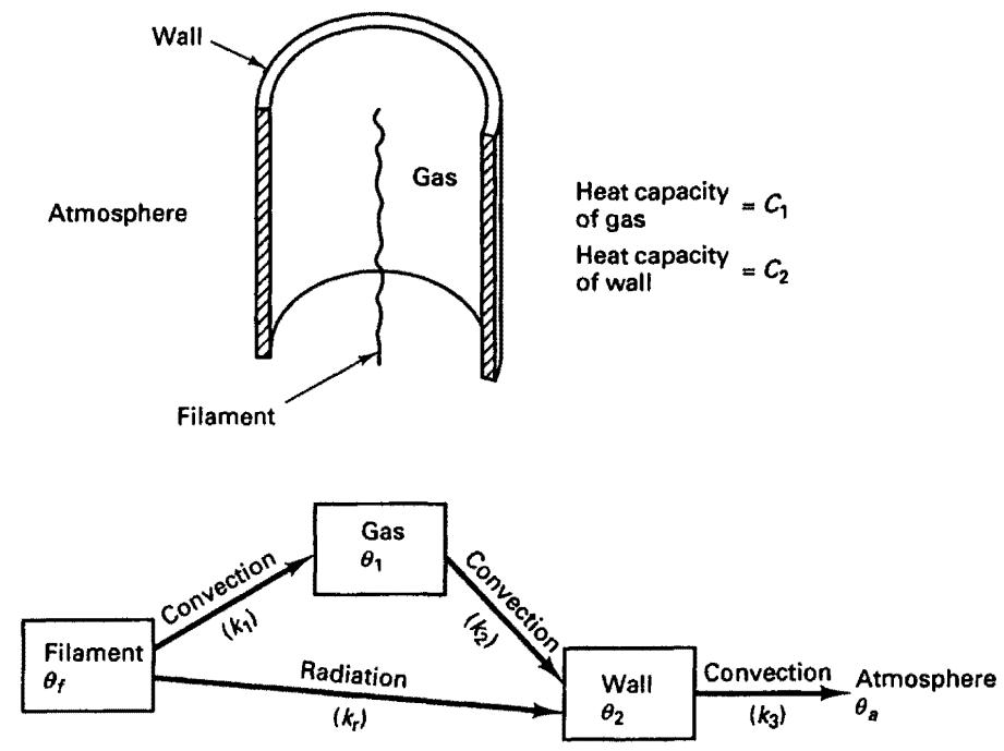EXAMPLE 3.9: Figure E3.9 shows an idealized case of the transient heat flow in an electron tube. A filament is heated to a temperature $\theta_{f}$ by an electric current; heat is convected from the filament to the surrounding gas and is radiated to the wall, which also receives heat by convection from the gas. The wall itself convects heat to the surrounding atmosphere, which is at temperature $\theta_{a}$ . It is required to formulate the system-governing heat flow equilibrium equations. In this analysis we choose as unknown state variables the temperature of the gas, $\theta_{1}$ , and the temperature of the wall, $\theta_{2}$ . The system equilibrium equations are generated by invoking the heat flow equilibrium for the gas and the wall. Using the heat transfer coefficients given in 

flowchart

```mermaid graph TD A["Atmosphere"] -->|Wall| B["Gas"] B -->|Heat capacity = C1| C["Heat capacity of gas"] B -->|Heat capacity = C2| D["Heat capacity of wall"] B --> E["Filament"] E --> F["Filament θf"] F -->|Convection (k1)| G["Gas θ1"] G -->|Convection (k2)| H["Wall θ2"] H -->|Convection (k3)| I["Atmosphere θa"] F -->|Radiation (kr)| H ```

Figure E3.9 Heat transfer idealization of an electron tube Fig. E3.9, we obtain for the gas $$ C _ {1} \frac {d \theta_ {1}}{d t} = k _ {1} (\theta_ {f} - \theta_ {1}) - k _ {2} (\theta_ {1} - \theta_ {2}) $$ and for the wall $$ C _ {2} \frac {d \theta_ {2}}{d t} = k _ {r} ((\theta_ {f}) ^ {4} - (\theta_ {2}) ^ {4}) + k _ {2} (\theta_ {1} - \theta_ {2}) - k _ {3} (\theta_ {2} - \theta_ {a}) $$ These two equations can be written in matrix form as where $\mathbf{C} = \begin{bmatrix} C_1 & 0 \\ 0 & C_2 \end{bmatrix}$ ; $\mathbf{K} = \begin{bmatrix} (k_1 + k_2) & -k_2 \\ -k_2 & (k_2 + k_3) \end{bmatrix}$ (a) $$ \boldsymbol {\theta} = \left[ \begin{array}{l} \theta_ {1} \\ \theta_ {2} \end{array} \right]; \quad \mathbf {Q} = \left[ \begin{array}{l} k _ {1} \theta_ {f} \\ k _ {r} ((\theta_ {f}) ^ {4} - (\theta_ {2}) ^ {4}) + k _ {3} \theta_ {a} \end{array} \right] $$ We note that because of the radiation boundary condition, the heat flow equilibrium equations are nonlinear in $\theta$ . Here the radiation boundary condition term has been incorporated in the heat flow load vector Q. The solution of the equations can be carried out as described in Section 9.6. Although, in the previous examples, we considered very specific cases, these examples illustrated in a quite general way how propagation problems of discrete systems are formu- lated for analysis. In essence, the same procedures are employed as in the analysis of steady-state problems, but “time-dependent loads” are generated that are a result of the “resistance to change” of the elements and thus of the complete system. This resistance to change or inertia of the system must be considered in a dynamic analysis. Based on the preceding arguments and observations, it appears that we can conclude that the analysis of a propagation problem is a very simple extension of the analysis of the corresponding steady-state problem. However, we assumed in the earlier discussion that the discrete system is given and thus the degrees of freedom or state variables can be directly identified. In practice, the selection of an appropriate discrete system that contains all the important characteristics of the actual physical system is usually not straightforward, and in general a different discrete model must be chosen for a dynamic response prediction than is chosen for the steady-state analysis. However, the discussion illustrates that once the discrete model has been chosen for a propagation problem, formulation of the governing equilibrium equations can proceed in much the same way as in the analysis of a steady-state response, except that inertia loads are generated that act on the system in addition to the externally applied loads (see Section 4.2.1). This observation leads us to anticipate that the procedures for solving the dynamic equilibrium equations of a system are largely based on the techniques employed for the solution of steady-state equilibrium equations (see Section 9.2). # 3.2.3 Eigenvalue Problems In our earlier discussion of steady-state and propagation problems we implied the existence of a unique solution for the response of the system. A main characteristic of an eigenvalue problem is that there is no unique solution to the response of the system, and the objective of the analysis is to calculate the various possible solutions. Eigenvalue problems arise in both steady-state and dynamic analyses. Various different eigenvalue problems can be formulated in engineering analysis. In this book we are primarily concerned with the generalized eigenvalue problem of the form $$ \mathbf {A} \mathbf {v} = \lambda \mathbf {B} \mathbf {v} \tag {3.5} $$ where $\mathbf{A}$ and $\mathbf{B}$ are symmetric matrices, $\lambda$ is a scalar, and $\mathbf{v}$ is a vector. If $\lambda_{i}$ and $\mathbf{v}_i$ satisfy (3.5), they are called an eigenvalue and an eigenvector, respectively. In steady-state analysis an eigenvalue problem of the form (3.5) is formulated when it is necessary to investigate the physical stability of the system under consideration. The question that is asked and leads to the eigenvalue problem is as follows: Assuming that the steady-state solution of the system is known, is there another solution into which the system could bifurcate if it were slightly perturbed from its equilibrium position? The answer to this question depends on the system under consideration and the loads acting on the system. We consider a very simple example to demonstrate the basic idea. 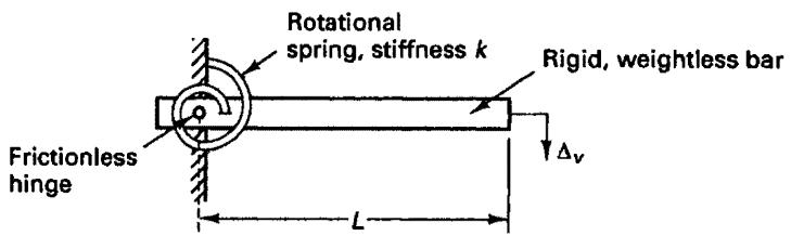EXAMPLE 3.10: Consider the simple cantilever shown in Fig. E3.10. The structure consists of a rotational spring and a rigid lever arm. Predict the response of the structure for the load applications shown in the figure. We consider first only the steady-state response as discussed in Section 3.2.1. Since the bar is rigid, the cantilever is a single degree of freedom system and we employ $\Delta_{v}$ as the state variable. 

text_image

Rotational spring, stiffness k Rigid, weightless bar Frictionless hinge L Δv

(a) Cantilever beam 

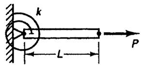
text_image

k L P

(1) 

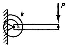
text_image

k P

(11) 

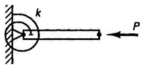
text_image

k P

(III) (b) Loading conditions 

text_image

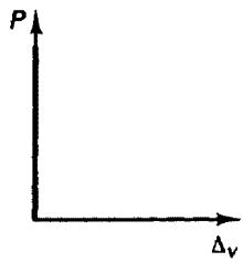
P Δv

(1) 

text_image

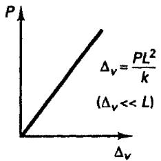
P Δv = PL²/k (Δv << L) Δv

(II) 

text_image

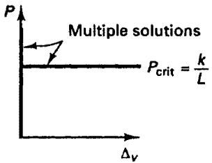
Multiple solutions P Pcrit = k/L Δv

(III) (c) Displacement responses 

text_image

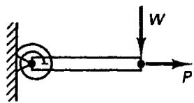
W P

(1) 

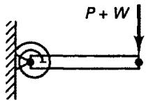
text_image

P + W

(II) 

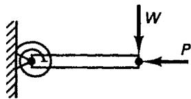
text_image

W P

(III) (d) Loading conditions (small load W) 

line

| Δv | P | | ---- | ----- | | Left | High | | Right| Low |

$\Delta_{v}$ due to $W$ at $P = 0$ $$ \Delta_ {v} = \frac {W L}{\left(\frac {k}{L} + P\right)} $$ (1) 

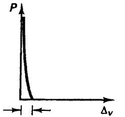
text_image

P P only P and W Δv

$\Delta_{\nu}$ due to $W$ at $P = 0$ $$ \Delta_ {v} = \frac {(P + W) L}{\left(\frac {k}{L}\right)} $$ (11) 

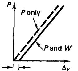
line

| Δv | P | | ---- | ----- | | < Δv | 0 | | > Δv | P_crit |

$\Delta_{\nu}$ due to $W$ at $P = 0$ $$ \Delta_ {v} = \frac {W L}{\left(\frac {k}{L} - P\right)} \text { for } P < P _ {\text { crit }} $$ (III) (e) Displacement responses Figure E3.10 Analysis of a simple cantilever model In loading condition I, the bar is subjected to a longitudinal tensile force P, and the moment in the spring is zero. Since the bar is rigid, we have $$ \Delta_ {v} = 0 \tag {a} $$ Next consider loading condition II. Assuming small displacements we have in this case $$ \Delta_ {v} = \frac {P L ^ {2}}{k} \tag {b} $$ Finally, for loading condition III we have, as in condition I, $$ \Delta_ {v} = 0 \tag {c} $$ We now proceed to determine whether the system is stable under these load applications. To investigate the stability we perturb the structure from the equilibrium positions defined in (a), (b), and (c) and ask whether an additional equilibrium position is possible. Assume that $\Delta_{v}$ is positive but small in loading conditions I and II. If we write the equilibrium equations taking this displacement into account, we observe that in loading condition I the small nonzero $\Delta_{v}$ cannot be sustained, and that in loading condition II the effect of including $\Delta_{v}$ in the analysis is negligible. Consider next that $\Delta_{v}>0$ in loading condition III. In this case, for an equilibrium configuration to be possible with $\Delta_{v}$ nonzero, the following equilibrium equation must be satisfied: $$ P \Delta_ {v} = k \frac {\Delta_ {v}}{L} $$ But this equation is satisfied for any $\Delta_{v}$ , provided P = k/L. Hence the critical load $P_{crit}$ at which an equilibrium position in addition to the horizontal one becomes possible is $$ P _ {\mathrm{crit}} = \frac {k}{L} $$ In summary, we have $$ P < P _ {\text { crit }} \quad \text { only the horizontal position of the bar is possible; equilibrium is stable } $$ $$ \begin{array}{l l} P = P _ {\text { crit }} & \text { horizontal and deflected positions of the bar are } \\ & \text { possible; the horizontal equilibrium position is } \\ & \text { unstable for } P \geq P _ {\text { crit }}. 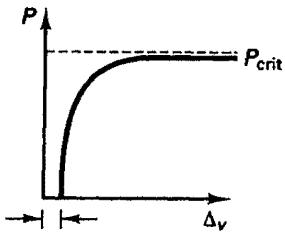\end{array} $$ To gain an improved understanding of these results we may assume that in addition to the load P shown in Fig. E3.10(b), a small transverse load W is applied as shown in Fig. E3.10(d). If we then perform an analysis of the cantilever model subjected to P and W, the response curves shown schematically in Fig. E3.10(e) are obtained. Thus, we observe that the effect of the load W decreases and is constant as P increases in loading conditions I and II, but that in loading condition III the transverse displacement $\Delta_{v}$ increases very rapidly as P approaches the critical load, $P_{crit}$ . The analyses given in Example 3.10 illustrate the main objective of an eigenvalue formulation and solution in instability analysis, namely, to predict whether small disturbances that are imposed on the given equilibrium configuration tend to increase very substantially. The load level at which this situation arises corresponds to the critical loading of the system. In the second solution carried out in Example 3.10 the small disturbance was due to the small load W, which, for example, may simulate the possibility that the horizontal load on the cantilever is not acting perfectly horizontally. In the eigenvalue analysis, we simply assume a deformed configuration and investigate whether there is a load level that indeed admits such a configuration as a possible equilibrium solution. We shall discuss in Section 6.8.2 that the eigenvalue analysis really consists of a linearization of the nonlinear response of the system, and that it depends largely on the system being considered whether a reliable critical load is calculated. The eigenvalue solution is particularly applicable in the analysis of “beam-column-type situations” of beam, plate, and shell structures. EXAMPLE 3.11: Experience shows that in structural analysis the critical load on column-type structures can be assessed appropriately using an eigenvalue problem formulation. Consider the system defined in Fig. E3.11. Construct the eigenvalue problem from which the critical loading on the system can be calculated.  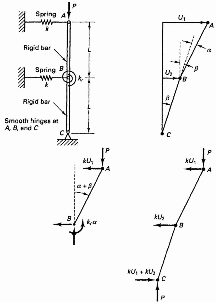Figure E3.11 Instability analysis of a column