and $U_{3} = \overline{V}_{3}^{(3)} = 292$ For $i = 3$ , $\overline{V}_2^{(2)} = \overline{V}_2^{(3)} - l_{23}U_3 = 35 - (-2)(292) = 619$ and $U_{2} = \overline{V}_{2}^{(2)} = 619$ For $i = 2$ , $\overline{V}_1^{(1)} = \overline{V}_1^{(2)} - l_{12}U_2 = 17 - (-1)(619) = 636$ and $U_{1} = \overline{V}_{1}^{(1)} = 636$ The elements stored in the vector that initially stored the loads are after step i = 5, 4, 3, 2, respectively: $$ \left[ \begin{array}{l} 1 7 \\ 3 5 \\ 7 0 \\ 7 4 \\ 3 4 \end{array} \right]; \quad \left[ \begin{array}{l} 1 7 \\ 3 5 \\ 2 9 2 \\ 7 4 \\ 3 4 \end{array} \right]; \quad \left[ \begin{array}{l} 1 7 \\ 6 1 9 \\ 2 9 2 \\ 7 4 \\ 3 4 \end{array} \right]; \quad \left[ \begin{array}{l} 6 3 6 \\ 6 1 9 \\ 2 9 2 \\ 7 4 \\ 3 4 \end{array} \right] $$ where the last vector gives the solution U. Considering the effectiveness of the active column solution algorithm, it should be noted that for a specific matrix K the algorithm frequently gives an efficient solution because no operations are performed on zero elements outside the skyline, which also implies that only the elements below the skyline need be stored. However, the total number of operations performed is not an absolute minimum because, in addition, all those multiplications could be skipped in (8.21) to (8.25) for which $l_{ri}$ or $g_{rj}$ is zero. This skipping of course requires additional logic, but is effective if there are many such cases, which is the main premise on which sparse solvers are based. These solvers, which can be very effective in large three-dimensional solutions, avoid the storage of elements that remain zero and skip the relevant operations, see, for example, A. George, J. R. Gilbert, and J. W. H. Liu (eds.) [A]. To evaluate the efficiency of the active column solution, let us consider a system with constant column heights, i.e. a half-bandwidth $m_{K}$ such that $m_{K} = i - m_{i}$ for all i, $i > m_{K}$ , and perform an operation count based on (8.16) to (8.25). We define one operation to consist of one multiplication (or division), which is nearly always followed by an addition. In this case the number of operations required for the $LDL^{T}$ decomposition of K are approximately $n[m_{K} + (m_{K} - 1) + \cdots + 1] = \frac{1}{2} nm_{K}^{2}$ , and for the reduction and back-substitution of a load vector, an additional number of approximately $2nm_{K}$ operations are needed. In practice, systems with exactly constant column heights are encountered rather seldom and therefore these operation counts should be refined to $\frac{1}{2} \Sigma_{i} (i - m_{i})^{2}$ and $2 \Sigma_{i} (i - m_{i})$ , respectively. However, we frequently still use the constant half-bandwidth formulas with a mean or effective half-bandwidth merely to obtain an indication of the required solution effort. Since the number of operations is governed by the pattern of the nonzero elements in the matrix, algorithms have been developed that reorder the equations so as to increase the effectiveness of the equation solution. When the active column solution scheme is used, the reordering is to reduce the column heights for an effective solution (see E. Cuthill and J. McKee [A] and N. E. Gibbs, W. G. Poole, Jr., and P. K. Stockmeyer [A]), while when a sparse solver is used the reordering is to reduce the total number of operations taking due account of not operating on elements that remain zero throughout the solution. This requirement for a sparse solver means that the number of fill-in elements (elements that originally are zero but become nonzero) should be small (see A. George, J. R. Gilbert, and J. W. H. Liu (eds.) [A]). The use of such reordering procedures, while generally not giving the actual optimal ordering of the equations, is very important because in practice the initial ordering of the equations is usually generated without regard to the efficiency of the equation solution but merely with regard to the effectiveness of the definition of the model. The solution algorithm in (8.21) to (8.25) has been presented in two-dimensional matrix notation; e.g., element $(r,j)$ of K has been denoted by $k_{rj}$ . Also, to demonstrate the working of the algorithm, in Examples 8.4 and 8.5 the elements considered in the reduction have been displayed in their corresponding matrix locations. However, in actual computer solution, the active columns of the matrix K are stored effectively in a one-dimensional array. Assume that the storage scheme discussed in Chapter 12 is used; i.e., the pertinent elements of K are stored in the one-dimensional array A of length NWK and the addresses of the diagonal elements of K are stored in MAXA. An effective subroutine that uses the algorithm presented above [i.e., the relations in (8.21) to (8.25)] but operates on the stiffness matrix using this storage scheme is given next. Subroutine COLSOL. Program COLSOL is an active column solver to obtain the $LDL^{T}$ factorization of a stiffness matrix or reduce and back-substitute the load vector. The complete process gives the solution of the finite element equilibrium equations. The argument variables and use of the subroutine are defined by means of comments in the program. ```csv SUBROUTINE COLSOL (A,V,MAXA,NN,NWK,NNM,KKK,IOUT) COL00001 C . . . . . . . . . . . . . . . . . . . . . . . . . . . . . . . . . . . . . . . . . . . . . . . . . . . . . . . . . . . . . . . . . . . . . . . . . . . . . . . . . . . . . . . . . . . . . . . . . . . . . C . . . . . . . . . . . . . . . . . . . . . . . . . . . . . . . . . . . . . . . . . . . . . . . . . . . . . . . . . . . . . . . . . . . . . . . . . . . . . . . . . . . . . . . . . . . . . . . . . . . P R O G R A M . . . . . . . . . . . . . . . . . . . . . . . . . . . . . . . . . . . . . . . . . . . . . . . . . . . . . . . . . . . . . . . . . . . . . . . . . . . . . . . . . . . . . . . . . . . . . . . . . . . C . . . . . . . . . . . . . . . . . . . . . . . . . . . . . . . . . . . . . . . . . . . . . . . . . . . . . . . . . . . . . . . . . . . . . . . . . . . . . . . . . . . . . . . . . . . . . . . . . . . - - INPUT VARIABLES - - . . . . . . . . . . . . . . . . . . . . . . . . . . . . . . . . . . . . . . . . . . . . . . . . . . . . . . . . . . . . . . . . . . . . . . . . . . . . . . . . . . . . . . . . . . . . . . . . . . . A(NWK) = STIFFNESS MATRIX STORED IN COMPACTED FORM . . . . . . . . . . . . . . . . . . . . . . . . . . . . . . . . . . . . . . . . . . . . . . . . . . . . . . . . . . . . . . . . . . . . . . . . . . . . . . . . . . . . . . . . . . . . . . . . . . . V(NN) = RIGHT-HAND-SIDE LOAD VECTOR . . . . . . . . . . . . . . . . . . . . . . . . . . . . . . . . . . . . . . . . . . . . . . . . . . . . . . . . . . . . . . . . . . . . . . . . . . . . . . . . . . . . . . . . . . . . . . . . . . . MAXA(NNM) = VECTOR CONTAINING ADDRESSES OF DIAGONAL . . . . . . . . . . . . . . . . . . . . . . . . . . . . . . . . . . . . . . . . . . . . . . . . . . . . . . . . . . . . . . . . . . . . . . . . . . . . . . . . . . . . . . . . . . . . . . . . . . . N N = NUMBER OF EQUATIONS . . . . . . . . . . . . . . . . . . . . . . . . . . . . . . . . . . . . . . . . . . . . . . . . . . . . . . . . . . . . . . . . . . . . . . . . . . . . . . . . . . . . . . . . . . . . . . . . . . . NWK = NUMBER OF ELEMENTS BELOW SKYLINE OF MATRIX . . . . . . . . . . . . . . . . . . . . . . . . . . . . . . . . . . . . . . . . . . . . . . . . . . . . . . . . . . . . . . . . . . . . . . . . . . . . . . . . . . . . . . . . . . . . . . . . . . . NN = NUMBER OF ELEMENTS BELOW SKYLINE OF MATRIX . . . . . . . . . . . . . . . . . . . . . . . . . . . . . . . . . . . . . . . . . . . . . . . . . . . . . . . . . . . . . . . . . . . . . . . . . . . . . . . . . . . . . . . . N N = NUMBER OF ELEMENTS BELOW SKYLINE OF MATRIX . . . . . . . . . . . . . . . . . . . . . . . . . . . . . . . . . . . . . . . . . . . . . . . . . . . . . . . . . . . . . . . . . . . . . . . . . . . . . . . . . . . . . . . . .. . . . . . . . . . . . . . . . . . . . . . . . . . . . . . . . . . . . . . . . . . . . . . . . . . . . . . . . . . . . . . . . . . . . . . . . . . . . . . . . . . . . . . . . . . . . . . . . . . . . .. . . . . . . . . . . .. . . . . . . . . . . . . . . . . . . . . . . . . . . . . . . . . . . . . . . . . . . . . . . . . . . . . . . . . . . . . . . . . . . . . . . . . . . . . . . . . . . . . . . . . .. . . . . . . . . . . 1000012 . . . . . . . . . . . . . . . . . . . . . . . . . . . . . . . . . . . . . . . . . . . . . . . . . . . . . . . . . . . . . . . . . . . . . . . . . . . . . . . . . . . . . . . . . . . . . . . . . . . 1000012 . . . . . . . . . . . . . . . . . . . . . . . . . . . . . . . . . . . . . . . . . . . . . . . . . . . . . . . . . . . . . . . . . . . . . . . . . . . . . . . . . 1000012 . . . . . . . . . . 1000012 . . . . . . . . . . . . . . . . . . . . . . . . . . . . . . . . . . . . . . . . . . . . . . . . . . . . . . . . . . . . . . . . . . . . . . . . . . . . . . . . . .. . . . . . . . . . . . . . . . . . 1000012 . . . . . . . . . . . . . . . . . . . . . . . . . . . . . . . . . . . . . . . . . . . . . . . . . . . . . . . . . . . . . . . . . . . . . . . . . . 1000012 . . . . . . . . . . . . . . . . . 1000012 . . . . . . . . . . . . . . . . . . . . . . . . . . . . . . . . . . . . . . . . . . . . . . . . . . . . . . . . . . . . . . . . . . . . . . . . . . .. . . . . . . . . . . . . . . . . . . . . . . . . 1000012 . . . . . . . . . . . . . . . . . . . . . . . . . . . . . . . . . . . . . . . . . . . . . . . . . . . . . . . . . . . . . . . . . . . 1000012 . . . . . . . . . . . . . . . . . . . . . . . . 1000012 . . . . . . . . . . . . . . . . . . . . . . . . . . . . . . . . . . . . . . . . . . . . . . . . . . . . . . . . . . . . . . . . . . . .. . . . . . . . . . . . . . . . . . . . . . . . . . . . . . . . 1000012 . . . . . . . . . . . . . . . . . . . . . . . . . . . . . . . . . . . . . . . . . . . . . . . . . . . . . . . . . . . . 1000012 . . . . . . . . . . . . . . . . . . . . . . . . . . . . . . . 1000012 . . . . . . . . . . . . . . . . . . . . . . . . . . . . . . . . . . . . . . . . . . . . . . . . . . . . . . . . . . . . .. . . . . . . . . . . . . . . . . . . . . . . . . . . . . . . . . . . . . . . 1000012 . . . . . . . . . . . . . . . . . . . . . . . . . . . . . . . . . . . . . . . . . . . . . . . . . . . . . 1000012 . . . . . . . . . . . . . . . . . . . . . . . . . . . . . . . . . . . . . . 1000012 . . . . . . . . . . . . . . . . . . . . . . . . . . . . . . . . . . . . . . . . . . . . . . . . . . . . . .. . . . . . . . . . . . . . . . . . . . . . . . . . . . . . . . . . . . . . . . . . . . . . 1000012 . . . . . . . . . . . . . . . . . . . . . . . . . . . . . . . . . . . . . . . . . . . . . . 1000012 . . . . . . . . . . . . . . . . . . . . . . . . . . . . . . . . . . . . . . . . . . . . . 1000012 . . . . . . . . . . . . . . . . . . . . . . . . . . . . . . . . . . . . . . . . . . . . . . .. . . . . . . . . . . . . . . . . . . . . . . . . . . . . . . . . . . . . . . . . . . . . . . . . . . . . 1000012 . . . . . . . . . . . . . . . . . . . . . . . . . . . . . . . . . . . . . . . 1000012 . . . . . . . . . . . . . . . . . . . . . . . . . . . . . . . . . . . . . . . . . . . . . . . . . . . . 1000012 . . . . . . . . . . . . . . . . . . . . . . . . . . . . . . . . . . . . . . . .. . . . . . . . . . . . . . . . . . . . . . . . . . . . . . . . . . . . . . . . . . . . . . . . . . . . . . . . . . . . 1000012 . . . . . . . . . . . . . . . . . . . . . . . . . . . . . . . . 1000012 . . . . . . . . . . . . . . . . . . . . . . . . . . . . . . . . . . . . . . . . . . . . . . . . . . . . . . . . . . . 1000012 . . . . . . . . . . . . . . . . . . . . . . . . . . . . . . . . .. . . . . . . . . . . . . . . . . . . . . . . . . . . . . . . . . . . . . . . . . . . . . . . . . . . . . . . . . . . . . . . . . . . 1000012 . . . . . . . . . . . . . . . . . . . . . . . . . 1000012 . . . . . . . . . . . . . . . . . . . . . . . . . . . . . . . . . . . . . . . . . . . . . . . . . . . . . . . . . . . . . . . . . . 1000012 . . . . . . . . . . . . . . . . . . . . . . . . . .. . . . . . . . . . . . . . . . . . . . . . . . . . . . . . . . . . . . . . . . . . . . . . . . . . . . . . . . . . . . . . . . . . . . . . . . . . 1000012 . . . . . . . . . . . . . . . . . . 1000012 . . . . . . . . . . . . . . . . . . . . . . . . . . . . . . . . . . . . . . . . . . . . . . . . . . . . . . . . . . . . . . . . . . . . . . . . . 1000012 . . . . . . . . . . . . . . . . . . .. . . . . . . . . . . . . . . . . . . . . . . . . . . . . . . . . . . . . . . . . . . . . . . . . . . . . . . . . . . . . . . . . . . . . . . . . . . . . . . . . 1000012 . . . . . . . . . . . 1000012 . . . . . . . . . . . . . . . . . . . . . . . . . . . . . . . . . . . . . . . . . . . . . . . . . . . . . . . . . . . . . . . . . . . . . . . . . . . . . . . . 1000012 . . . . . . . . . . . .. . . . . . . . . . . . . . . . . . . . . . . . . . . . . . . . . . . . . . . . . . . . . . . . . . . . . . . . . . . . . . . . . . . . . . . . . . . . . . . . . . . . . . . . 1000012 . . . . 1000012 . . . . . . . . . . . . . . . . . . . . . . . . . . . . . . . . . . . . . . . . . . . . . . . . . . . . . . . . . . . . . . . . . . . . . . . . . . . . . . . . . . . . . . . 1000012 . . . . .. . . . . . . . . . . . . . . . . . . . . . . . . . . . . . . . . . . . . . . . . . . . . . . . . . . . . . . . . . . . . . . . . . . . . . . . . . . . . . . . . . . . . . . . . . . . . . . 100012 . . . . . . . . . . . . . . . . . . . . . . . . . . . . . . . . . . . . . . . . . . . . . . . . . . . . . . . . . . . . . . . . . . . . . . . . . . . . . . . . . . . . . . . . . . . . . . 100022 . . . . . . . . . . . . . . . . . . . . . . . . . . . . . . . . . . . . . . . . . . . . . . . . . . . . . . . . . . . . . . . . . . . . . . . . . . . . . . . . . . . . . . . . . . . . . . . . . . 200012 . . . . . . . . . . . . . . . . . . . . . . . . . . . . . . . . . . . . . . . . . . . . . . . . . . . . . . . . . . . . . . . . . . . . . . . . . . . . . . . . . . . . . . . . . . . . . . .. . . . . 1000012 . . . . . . . . . . . . . . . . . . . . . . . . . . . . . . . . . . . . . . . . . . . . . . . . . . . . . . . . . . . . . . . . . . . . . . . . . . . . . . . . . . . . . . . .. . . . . . . . . . . . 1000012 . . . . . . . . . . . . . . . . . . . . . . . . . . . . . . . . . . . . . . . . . . . . . . . . . . . . . . . . . . . . . . . . . . . . . . . . . . . . . . . . .. . . . . . . . . . . . . . . . . . . 1000012 . . . . . . . . . . . . . . . . . . . . . . . . . . . . . . . . . . . . . . . . . . . . . . . . . . . . . . . . . . . . . . . . . . . . . . . . . .. . . . . . . . . . . . . . . . . . . . . . . . . . 1000012 . . . . . . . . . . . . . . . . . . . . . . . . . . . . . . . . . . . . . . . . . . . . . . . . . . . . . . . . . . . . . . . . . . .. . . . . . . . . . . . . . . . . . . . . . . . . . . . . . . . . 1000012 . . . . . . . . . . . . . . . . . . . . . . . . . . . . . . . . . . . . . . . . . . . . . . . . . . . . . . . . . . . .. . . . . . . . . . . . . . . . . . . . . . . . . . . . . . . . . . . . . . . . 1000012 . . . . . . . . . . . . . . . . . . . . . . . . . . . . . . . . . . . . . . . . . . . . . . . . . . . . .. . . . . . . . . . . . . . . . . . . . . . . . . . . . . . . . . . . . . . . . . . . . . . . 1000012 . . . . . . . . . . . . . . . . . . . . . . . . . . . . . . . . . . . . . . . . . . . . . .. . . . . . . . . . . . . . . . . . . . . . . . . . . . . . . . . . . . . . . . . . . . . . . . . . . . . . 1000012 . . . . . . . . . . . . . . . . . . . . . . . . . . . . . . . . . . . . . . .. . . . . . . . . . . . . . . . . . . . . . . . . . . . . . . . . . . . . . . . . . . . . . . . . . . . . . . . . . . . . 1000012 . . . . . . . . . . . . . . . . . . . . . . . . . . . . . . . .. . . . . . . . . . . . . . . . . . . . . . . . . . . . . . . . . . . . . . . . . . . . . . . . . . . . . . . . . . . . . . . . . . . . 1000012 . . . . . . . . . . . . . . . . . . . . . . . . .. . . . . . . . . . . . . . . . . . . . . . . . . . . . . . . . . . . . . . . . . . . . . . . . . . . . . . . . . . . . . . . . . . . . . . . . . . . 1000012 . . . . . . . . . . . . . . . . . .. . . . . . . . . . . . . . . . . . . . . . . . . . . . . . . . . . . . . . . . . . . . . . . . . . . . . . . . . . . . . . . . . . . . . . . . . . . . . . . . . . 1000012 . . . . . . . . . . .. . . . . . . . . . . . . . . . . . . . . . . . . . . . . . . . . . . . . . . . . . . . . . . . . . . . . . . . . . . . . . . . . . . . . . . . . . . . . . . . . . . . . . . . . 1000012 . . . .. . . . . . . . . . . . . . . . . . . . . . . . . . . . . . . . . . . . . . . . . . . . . . . . . . . . . . . . . . . . . . . . . . . . . . . . . . . . . . . . . . . . . . . . . . . . . . . . 100122 . . . . . . . . . . . . . . . . . . . . . . . . . . . . . . . . . . . . . . . . . . . . . . . . . . . . . . . . . . . . . . . . . . . . . . . . . . . . . . . . . . . . . . . . . . . . . . . . . 1100012 . . . . . . . . . . . . . . . . . . . . . . . . . . . . . . . . . . . . . . . . . . . . . . . . . . . . . . . . . . . . . . . . . . . . . . . . . . . . . . . . . . . . . . . . . . . . . 1000022 . . . . . . . . . . . . . . . . . . . . . . . . . . . . . . . . . . . . . . . . . . . . . . . . . . . . . . . . . . . . . . . . . . . . . . . . . . . . . . . . . . . . . . . . . . . . . . 1001122 . . . . . . . . . . . . . . . . . . . . . . . . . . . . . . . . . . . . . . . . . . . . . . . . . . . . . . . . . . . . . . . . . . . . . . . . . . . . . . . . . . . . . . . . . . . . . . . . 101122 . . . . . . . . . . . . . . . . . . . . . . . . . . . . . . . . . . . . . . . . . . . . . . . . . . . . . . . . . . . . . . . . . . . . . . . . . . . . . . . . . . . . . . . . . . . . . . 1011122 . . . . . . . . . . . . . . . . . . . . . . . . . . . . . . . . . . . . . . . . . . . . . . . . . . . . . . . . . . . . . . . . . . . . . . . . . . . . . . . . . . . . . . . . . . . . . . . 10101122 . . . . . . . . . . . . . . . . . . . . . . . . . . . . . . . . . . . . . . . . . . . . . . . . . . . . . . . . . . . . . . . . . . . . . . . . . . . . . . . . . . . . . . . . . . . . . 1010122 . . . . . . . . . . . . . . . . . . . . . . . . . . . . . . . . . . . . . . . . . . . . . . . . . . . . . . . . . . . . . . . . . . . . . . . . . . . . . . . . . . . . . . . . . . . . . . . 2010122 . . . . . . . . . . . . . . . . . . . . . . . . . . . . . . . . . . . . . . . . . . . . . . . . . . . . . . . . . . . . . . . . . . . . . . . . . . . . . . . . . . . . . . . . . . . . . 10011122 . . . . . . . . . . . . . . . . . . . . . . . . . . . . . . . . . . . . . . . . . . . . . . . . . . . . . . . . . . . . . . . . . . . . . . . . . . . . . . . . . . . . . . . . . . . . . 11011122 . . . . . . . . . . . . . . . . . . . . . . . . ``` ```csv KU=MAXA(N+1) - 1 KH=KU - KL IF (KH) 110,90,50 50 K=N - KH IC=0 KLT=KU DO 80 J=1,KH IC=IC + 1 KLT=KLT - 1 KI=MAXA(K) ND=MAXA(K+1) - KI - 1 IF (ND) 80,80,60 60 KK=MIN0(IC,ND) C=0. DO 70 L=1,KK 70 C=C + A(KI+L)*A(KLT+L) A(KLT)=A(KLT) - C 80 K=K + 1 90 K=N B=0. DO 100 KK=KL,KU K=K - 1 KI=MAXA(K) C=A(KK)/A(KI) B=B + C*A(KK) 100 A(KK)=C A(KN)=A(KN) - B 110 IF (A(KN)) 120,120,140 120 WRITE (IOUT,2000) N,A(KN) GO TO 800 140 CONTINUE GO TO 900 C REDUCE RIGHT-HAND-SIDE LOAD VECTOR C 150 DO 180 N=1,NN KL=MAXA(N) + 1 KU=MAXA(N+1) - 1 IF (KU-KL) 180,160,160 160 K=N C=0. DO 170 KK=KL,KU K=K - 1 170 C=C + A(KK)*V(K) V(N)=V(N) - C 180 CONTINUE C BACK-SUBSTITUTE C DO 200 N=1,NN K=MAXA(N) 200 V(N)=V(N)/A(K) IF (NN.EQ.1) GO TO 900 N=NN DO 230 L=2,NN KL=MAXA(N) + 1 KU=MAXA(N+1) - 1 IF (KU-KL) 230,210,210 210 K=N DO 220 KK=KL,KU K=K - 1 220 V(K)=V(K) - A(KK)*V(N) 230 N=N - 1 GO TO 900 C 800 STOP 900 RETURN C 2000 FORMAT (//' STOP - STIFFNESS MATRIX NOT POSITIVE DEFINITE',//, 1 ' NONPOSITIVE PIVOT FOR EQUATION ',I8,//, 2 ' PIVOT = ',E20.12 ) END COL00041 COL00042 COL00043 COL00044 COL00045 COL00046 COL00047 COL00048 COL00049 COL00050 COL00051 COL00052 COL00053 COL00054 COL00055 COL00056 COL00057 COL00058 COL00059 COL00060 COL00061 COL00062 COL00063 COL00064 COL00065 COL00066 COL00067 COL00068 COL00069 COL00070 COL00071 COL00072 COL00073 COL00074 COL00075 COL00076 COL00077 COL00078 COL00079 COL00080 COL00081 COL00082 COL00083 COL00084 COL00085 COL00086 COL00087 COL00088 COL00089 COL00090 COL00091 COL00092 COL00093 COL00094 COL00095 COL00096 COL00097 COL00098 COL00099 COL00100 COL00101 COL00102 COL00103 COL00104 COL00105 COL00106 COL00107 COL00108 COL00109 COL00110 COL00111 COL00112 ``` # 8.2.4 Cholesky Factorization, Static Condensation, Substructures, and Frontal Solution In addition to the $LDL^{T}$ decomposition described in the preceding sections, various other schemes are used that are closely related. All methods are applications of the basic Gauss elimination procedure. In the Cholesky factorization the stiffness matrix is decomposed as follows: $$ \mathbf {K} = \tilde {\mathbf {L}} \tilde {\mathbf {L}} ^ {T} \tag {8.26} $$ where $$ \tilde {\mathbf {L}} = \mathbf {L} \mathbf {D} ^ {1 / 2} \tag {8.27} $$ Therefore, the Cholesky factors could be calculated from the D and L factors, but, more generally, the elements of $\tilde{L}$ are calculated directly. An operation count shows that slightly more operations are required in the equation solution if the Cholesky factorization is used rather than the $LDL^{T}$ decomposition. In addition, the Cholesky factorization is suitable only for the solution of positive definite systems, for which all diagonal elements $d_{ii}$ are positive, because otherwise complex arithmetic would be required. On the other hand, the $LDL^{T}$ decomposition can also be used effectively on indefinite systems (see Section 8.2.5). Considering a main use of the Cholesky factorization, the decomposition is employed effectively in the transformation of a generalized eigenproblem to the standard form (see Section 10.2.5). EXAMPLE 8.7: Calculate the Cholesky factor $\tilde{L}$ of the stiffness matrix K of the simply supported beam treated in Section 8.2.1 and in Examples 8.2 to 8.4. The L and D factors of the beam stiffness matrix have been given in Example 8.3. Rounding to three significant decimals, we have $$ \mathbf {L} = \left[ \begin{array}{c c c c} 1. 0 0 0 & & & \\ - 0. 8 0 0 & 1. 0 0 0 & 0 & \\ 0. 2 0 0 & - 1. 1 4 3 & 1. 0 0 0 & \\ 0. 0 0 0 & 0. 3 5 7 & - 1. 3 3 3 & 1. 0 0 0 \end{array} \right]; \quad \mathbf {D} = \left[ \begin{array}{c c c c} 5. 0 0 0 & & & \\ & 2. 8 0 0 & & \\ & & 2. 1 4 3 & \\ & & & 0. 8 3 3 \end{array} \right] $$ Hence, $$ \tilde {\mathbf {L}} = \left[ \begin{array}{c c c c} 1. 0 0 0 & & & \\ - 0. 8 0 0 & 1. 0 0 0 & & \\ 0. 2 0 0 & - 1. 1 4 3 & 1. 0 0 0 & \\ 0. 0 0 0 & 0. 3 5 7 & - 1. 3 3 3 & 1. 0 0 0 \end{array} \right] \left[ \begin{array}{c c c c} 2. 2 3 6 & & & \\ & 1. 6 7 3 & & \\ & & 1. 4 6 4 & \\ & & & 0. 9 1 3 \end{array} \right] $$ $$ \mathbf {L} = \left[ \begin{array}{c c c c} 2. 2 3 6 & & & \\ - 1. 7 8 9 & 1. 6 7 3 & & \\ 0. 4 4 7 & - 1. 9 1 2 & 1. 4 6 4 & \\ 0 & 0. 5 9 7 & - 1. 9 5 2 & 0. 9 1 3 \end{array} \right] $$ An algorithm that in some cases can effectively be used in the solution of the equilibrium equations is static condensation (see E. L. Wilson [B]). The name “static condensation” refers to dynamic analysis, for which the solution technique is demonstrated in Section 10.3.1. Static condensation is employed to reduce the number of element degrees of freedom and thus, in effect, to perform part of the solution of the total finite element system equilibrium equations prior to assembling the structure matrices K and R. Consider the three-node truss element in Example 8.8. Since the degree of freedom at the midnode does not correspond to a degree of freedom of any other element, we can eliminate it to obtain the element stiffness matrix that corresponds to the degrees of freedom 1 and 3 only. The elimination of the degree of freedom 2 is carried out using, in essence, Gauss elimination, as presented in Section 8.2.1 (see Example 8.1). In order to establish the equations used in static condensation, we assume that the stiffness matrix and corresponding displacement and force vectors of the element under consideration are partitioned into the form $$ \left[ \begin{array}{l l} \mathbf {K} _ {a a} & \mathbf {K} _ {a c} \\ \mathbf {K} _ {c a} & \mathbf {K} _ {c c} \end{array} \right] \left[ \begin{array}{l} \mathbf {U} _ {a} \\ \mathbf {U} _ {c} \end{array} \right] = \left[ \begin{array}{l} \mathbf {R} _ {a} \\ \mathbf {R} _ {c} \end{array} \right] \tag {8.28} $$ where $U_{a}$ and $U_{c}$ are the vectors of displacements to be retained and condensed out, respectively. The matrices $K_{aa}$ , $K_{ac}$ , and $K_{cc}$ and vectors $R_{a}$ and $R_{c}$ correspond to the displacement vectors $U_{a}$ and $U_{c}$ . Using the second matrix equation in (8.28), we obtain $$ \mathbf {U} _ {c} = \mathbf {K} _ {c c} ^ {- 1} (\mathbf {R} _ {c} - \mathbf {K} _ {c a} \mathbf {U} _ {a}) \tag {8.29} $$ The relation in (8.29) is used to substitute for $U_{c}$ into the first matrix equation in (8.28) to obtain the condensed equations $$ (\mathbf {K} _ {a a} - \mathbf {K} _ {a c} \mathbf {K} _ {c c} ^ {- 1} \mathbf {K} _ {c a}) \mathbf {U} _ {a} = \mathbf {R} _ {a} - \mathbf {K} _ {a c} \mathbf {K} _ {c c} ^ {- 1} \mathbf {R} _ {c} \tag {8.30} $$ Comparing (8.30) with the Gauss solution scheme introduced in Section 8.2.1, it is seen that static condensation is, in fact, Gauss elimination on the degrees of freedom $U_{c}$ (see Example 8.8). In practice, therefore, static condensation is carried out effectively by using Gauss elimination sequentially on each degree of freedom to be condensed out, instead of following through the formal matrix procedure given in (8.28) to (8.30), where it is valuable to keep the physical meaning of Gauss elimination in mind (see Section 8.2.1). Since the system stiffness matrix is obtained by direct addition of the element stiffness matrices, we realize that when condensing out internal element degrees of freedom, in fact, part of the total Gauss solution is already carried out on the element level. The advantage of using static condensation on the element level is that the order of the system matrices is reduced, which may mean that use of backup storage is prevented. In addition, if subsequent elements are identical, the stiffness matrix of only the first element needs to be derived, and performing static condensation on the element internal degrees of freedom also reduces the computer effort required. It should be noted, though, that if static condensation is actually carried out for each element (and no advantage is taken of possible identical finite elements), the total effort involved in the static condensation on all element stiffness matrices and in the Gauss elimination solution of the resulting assembled equilibrium equations is, in fact, the same as using Gauss elimination on the system equations established from the uncondensed element stiffness matrices. 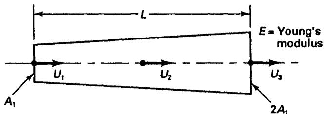EXAMPLE 8.8: The stiffness matrix of the truss element in Fig. E8.8 is given on the next page. Use static condensation as given in (8.28) to (8.30) to condense out the internal element degree of freedom. Then use Gauss elimination directly on the internal degree of freedom. 

text_image

L E = Young's modulus U₁ U₂ U₃ A₁ 2A₁

Figure E8.8 Truss element with linearly varying area We have for the element, $$ \frac {E A _ {1}}{6 L} \left[ \begin{array}{r r r} 1 7 & - 2 0 & 3 \\ - 2 0 & 4 8 & - 2 8 \\ 3 & - 2 8 & 2 5 \end{array} \right] \left[ \begin{array}{l} U _ {1} \\ U _ {2} \\ U _ {3} \end{array} \right] = \left[ \begin{array}{l} R _ {1} \\ R _ {2} \\ R _ {3} \end{array} \right] \tag {a} $$ In order to apply the equations in (8.28) to (8.30), we rearrange the equations in (a) to obtain $$ \frac {E A _ {1}}{6 L} \left[ \begin{array}{r r r} 1 7 & 3 & - 2 0 \\ 3 & 2 5 & - 2 8 \\ - 2 0 & - 2 8 & 4 8 \end{array} \right] \left[ \begin{array}{l} U _ {1} \\ U _ {3} \\ U _ {2} \end{array} \right] = \left[ \begin{array}{l} R _ {1} \\ R _ {3} \\ R _ {2} \end{array} \right] $$ The relation in (8.30) now gives $$ \frac {E A _ {1}}{6 L} \left\{\left[ \begin{array}{c c} 1 7 & 3 \\ 3 & 2 5 \end{array} \right] - \left[ \begin{array}{c} - 2 0 \\ - 2 8 \end{array} \right] \left[ \frac {1}{4 8} \right] \left[ \begin{array}{c c} - 2 0 & - 2 8 \end{array} \right] \right\} \left[ \begin{array}{c} U _ {1} \\ U _ {3} \end{array} \right] = \left[ \begin{array}{c} R _ {1} + \frac {2 0}{4 8} R _ {2} \\ R _ {3} + \frac {2 8}{4 8} R _ {2} \end{array} \right] $$ or $\frac{13}{9}\frac{EA_1}{L}\left[ \begin{array}{cc}1 & -1\\ -1 & 1 \end{array} \right]\left[ \begin{array}{l}U_1\\ U_3 \end{array} \right] = \left[ \begin{array}{ll}R_1 + \frac{5}{12} R_2\\ R_3 + \frac{7}{12} R_2 \end{array} \right]$ Also, (8.29) yields $U_{2} = \frac{1}{24}\left(\frac{3L}{EA_{1}} R_{2} + 10U_{1} + 14U_{3}\right)$ (b) Using Gauss elimination directly on (a) for $U_{2}$ , we obtain $$ \frac {E A _ {1}}{6 L} \left[ \begin{array}{c c c} 1 7 - \frac {(2 0) (2 0)}{4 8} & 0 & 3 - \frac {(2 0) (2 8)}{4 8} \\ - 2 0 & 4 8 & - 2 8 \\ 3 - \frac {(2 0) (2 8)}{4 8} & 0 & 2 5 - \frac {(2 8) (2 8)}{4 8} \end{array} \right] \left[ \begin{array}{l} U _ {1} \\ U _ {2} \\ U _ {3} \end{array} \right] = \left[ \begin{array}{c} R _ {1} + \frac {2 0}{4 8} R _ {2} \\ R _ {2} \\ R _ {3} + \frac {2 8}{4 8} R _ {2} \end{array} \right] \tag {c} $$ But separating the equations for $U_{1}$ and $U_{3}$ from the equation for $U_{2}$ , we can rewrite the relation in (c) as $$ \frac {1 3}{9} \frac {E A _ {1}}{L} \left[ \begin{array}{c c} 1 & - 1 \\ - 1 & 1 \end{array} \right] \left[ \begin{array}{l} U _ {1} \\ U _ {3} \end{array} \right] = \left[ \begin{array}{l} R _ {1} + \frac {5}{1 2} R _ {2} \\ R _ {3} + \frac {7}{1 2} R _ {2} \end{array} \right] $$ and $U_{2} = \frac{1}{24}\left[\frac{3L}{EA_{1}} R_{2} + 10U_{1} + 14U_{3}\right]$ which are the relations obtained using the formal static condensation procedure. 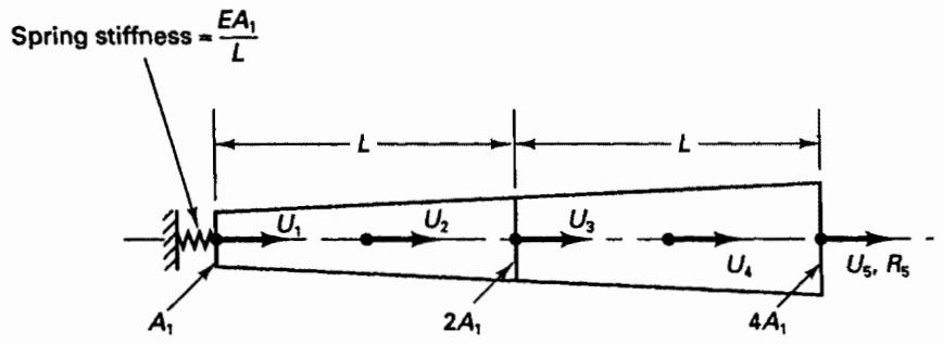EXAMPLE 8.9: Use the stiffness matrix of the three degree of freedom truss element in Example 8.8 to establish the equilibrium equations of the structure shown in Fig. E8.9. Use Gauss elimination directly on degrees of freedom $U_{2}$ and $U_{4}$ . Show that the resulting equilibrium equations are identical to those obtained when the two degree of freedom truss element stiffness matrix derived in Example 8.8 (the internal degree of freedom has been condensed out) is used to assemble the stiffness matrix corresponding to $U_{1}$ , $U_{3}$ , and $U_{5}$ . 

text_image

Spring stiffness = EA₁/L L L U₁ U₂ U₃ U₄ U₅, R₅ A₁ 2A₁ 4A₁

Figure E8.9 Structure composed of two truss elements of Fig. E8.8 and a spring support The stiffness matrix of the three-element assemblage in Fig. E8.9 is obtained using the direct stiffness method; i.e., we calculate $$ \mathbf {K} = \sum_ {m = 1} ^ {3} \mathbf {K} ^ {(m)} \tag {a} $$ where $\mathbf{K}^{(1)} = \frac{EA_1}{6L}\left[ \begin{array}{cccccc}6 & 0 & 0 & 0 & 0\\ 0 & 0 & 0 & 0 & 0\\ 0 & 0 & 0 & 0 & 0\\ 0 & 0 & 0 & 0 & 0\\ 0 & 0 & 0 & 0 & 0 \end{array} \right]$ $$ \mathbf {K} ^ {(2)} = \frac {E A _ {1}}{6 L} \left[ \begin{array}{c c c c c} 1 7 & - 2 0 & 3 & 0 & 0 \\ - 2 0 & 4 8 & - 2 8 & 0 & 0 \\ 3 & - 2 8 & 2 5 & 0 & 0 \\ 0 & 0 & 0 & 0 & 0 \\ 0 & 0 & 0 & 0 & 0 \end{array} \right] $$ $$ \mathbf {K} ^ {(3)} = \frac {E A _ {1}}{6 L} \left[ \begin{array}{c c c c c} 0 & 0 & 0 & 0 & 0 \\ 0 & 0 & 0 & 0 & 0 \\ 0 & 0 & 3 4 & - 4 0 & 6 \\ 0 & 0 & - 4 0 & 9 6 & - 5 6 \\ 0 & 0 & 6 & - 5 6 & 5 0 \end{array} \right] $$ Hence the equilibrium equations of the structure are $$ \frac {E A _ {1}}{6 L} \left[ \begin{array}{r r r r r} 2 3 & - 2 0 & 3 & 0 & 0 \\ - 2 0 & 4 8 & - 2 8 & 0 & 0 \\ 3 & - 2 8 & 5 9 & - 4 0 & 6 \\ 0 & 0 & - 4 0 & 9 6 & - 5 6 \\ 0 & 0 & 6 & - 5 6 & 5 0 \end{array} \right] \left[ \begin{array}{l} U _ {1} \\ U _ {2} \\ U _ {3} \\ U _ {4} \\ U _ {5} \end{array} \right] = \left[ \begin{array}{l} 0 \\ 0 \\ 0 \\ 0 \\ R _ {5} \end{array} \right] $$ Using Gauss elimination on degrees of freedom $U_{2}$ and $U_{4}$ , we obtain $$ \frac {E A _ {1}}{6 L} \left[ \begin{array}{c c c c c} 2 3 - \frac {(2 0) (2 0)}{4 8} & 0 & 3 - \frac {(2 0) (2 8)}{4 8} & 0 & 0 \\ - 2 0 & 4 8 & - 2 8 & 0 & 0 \\ 3 - \frac {(2 0) (2 8)}{4 8} & 0 & 5 9 - \frac {(2 8) (2 8)}{4 8} - \frac {(4 0) (4 0)}{9 6} & 0 & 6 - \frac {(4 0) (5 6)}{9 6} \\ 0 & 0 & - 4 0 & 9 6 & - 5 6 \\ 0 & 0 & 6 - \frac {(4 0) (5 6)}{9 6} & 0 & 5 0 - \frac {(5 6) (5 6)}{9 6} \end{array} \right] \left[ \begin{array}{l} U _ {1} \\ U _ {2} \\ U _ {3} \\ U _ {4} \\ U _ {5} \end{array} \right] = \left[ \begin{array}{l} 0 \\ 0 \\ 0 \\ 0 \\ R _ {5} \end{array} \right] \tag {b} $$ Now, extracting the equilibrium equations corresponding to degrees of freedom 1, 3, and 5 and degrees of freedom 2 and 4 separately, we have $$ \frac {1 3}{9} \frac {E A _ {1}}{L} \left[ \begin{array}{c c c} \frac {2 2}{1 3} & - 1 & 0 \\ - 1 & 3 & - 2 \\ 0 & - 2 & 2 \end{array} \right] \left[ \begin{array}{l} U _ {1} \\ U _ {3} \\ U _ {5} \end{array} \right] = \left[ \begin{array}{l} 0 \\ 0 \\ R _ {5} \end{array} \right] \tag {c} $$ and $U_{2} = \frac{1}{12} [5U_{1} + 7U_{3}]$ $$ U _ {4} = \frac {1}{1 2} \left[ 5 U _ {3} + 7 U _ {5} \right] \tag {d} $$ However, using the two degree of freedom truss element stiffness matrix derived in Example 8.8 to directly assemble the structure stiffness matrix corresponding to degrees of freedom 1, 3, and 5, we use as element stiffness matrices in (a), $$ \mathbf {K} ^ {(1)} = \frac {1 3}{9} \frac {E A _ {1}}{L} \left[ \begin{array}{l l l} \frac {9}{1 3} & 0 & 0 \\ 0 & 0 & 0 \\ 0 & 0 & 0 \end{array} \right] $$ $$ \mathbf {K} ^ {(2)} = \frac {1 3}{9} \frac {E A _ {1}}{L} \left[ \begin{array}{c c c} 1 & - 1 & 0 \\ - 1 & 1 & 0 \\ 0 & 0 & 0 \end{array} \right] \tag {e} $$ $$ \mathbf {K} ^ {(3)} = \frac {1 3}{9} \frac {E A _ {1}}{L} \left[ \begin{array}{c c c} 0 & 0 & 0 \\ 0 & 2 & - 2 \\ 0 & - 2 & 2 \end{array} \right] \tag {f} $$ and obtain the stiffness matrix in (c). Also, the relation (b) in Example 8.8 corresponds to relations (d) in this example. It should be noted that the total effort to solve the equilibrium equations using the condensed truss element stiffness matrix is less than when the original three degree of freedom element stiffness matrix is used because in the first case the internal degree of freedom was statically condensed out only once, whereas in (b) the element internal degree of freedom is, in fact, statically condensed out twice. The direct solution using the condensed element stiffness matrices in (e) and (f) is, however, possible only because these stiffness matrices are multiples of each other. As indicated in Example 8.9, it can be particularly effective to employ static condensation when the same element is used many times. An application of this concept is employed in substructure analysis, in which the total structure is considered to be an assemblage of substructures (see, for example, J. S. Przemieniecki [A] and M. F. Rubinstein [A]). Each substructure, in turn, is idealized as an assemblage of finite elements, and all internal degrees of freedom are statically condensed out. The total structure stiffness is formed by assembling the condensed substructure stiffness matrices. Therefore, in effect, a substructure is used in the same way as an individual finite element with internal degrees of freedom that are statically condensed out prior to the element assemblage process. If many substructures are identical, it is effective to establish a library of substructures from which a condensed total structure stiffness matrix is formed. It should be noted that the unreduced complete structure stiffness matrix is never calculated in substructure analysis, and input data are required only for each substructure in the library plus information on the assemblage of the substructures to make up the complete structure. Typical applications of finite element analysis using substructuring are found in the analysis of buildings and ship hulls, where the substructure technique has allowed economical analysis of very large finite element systems. The use of substructuring can also be effective in the analysis of structures with local nonlinearities in static and dynamic response calculations (see K. J. Bathe and S. Gracewski [A]). As a simple example of substructuring, we refer to Example 8.9, in which each substructure is composed simply of one element, and the uncondensed and condensed stiffness matrix of a typical substructure was given in Example 8.8. The effectiveness of analysis using the basic substructure concept described above can in many cases still be improved on by defining different levels of substructures; i.e., since each substructure can be looked on as a “super-finite element,” it is possible to define second, third, etc., levels of substructuring. In a similar procedure, two substructures are always combined to define the next-higher-level substructure until the final substructure is, in fact, the actual structure under consideration. The procedure may be employed in one-, two-, or three-dimensional analysis and, as pointed out earlier, is indeed only an effective application of Gauss elimination, in which advantage is taken of the repetition of submatrices, which are the stiffness matrices that correspond to the identical substructures. The possibility of using the solution procedure effectively therefore depends on whether the structure is made up of repetitive substructures, and this is the reason the procedure can be very effective in special-purpose programs. 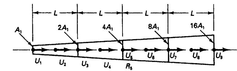EXAMPLE 8.10: Use substructuring to evaluate the stiffness matrix and the load vector corresponding to the end nodal point degrees of freedom $U_{1}$ and $U_{9}$ of the bar in Fig. E8.10. The basic element of which the bar is composed is the three degree of freedom truss element considered in Example 8.8. The equilibrium equations of the element corresponding to the two degrees of freedom $U_{1}$ and $U_{3}$ as shown in Fig. E8.10 are $$ \frac {1 3}{9} \frac {A _ {1} E}{L} \left[ \begin{array}{c c} 1 & - 1 \\ - 1 & 1 \end{array} \right] \left[ \begin{array}{l} U _ {1} \\ U _ {3} \end{array} \right] = \left[ \begin{array}{l} R _ {1} + \frac {5}{1 2} R _ {2} \\ R _ {3} + \frac {7}{1 2} R _ {2} \end{array} \right] \tag {a} $$ Since the internal degree of freedom $U_{2}$ has been statically condensed out to obtain the equilibrium relations in (a), we may regard the two degree of freedom element as a first-level substructure. We should recall that once $U_{1}$ and $U_{3}$ have been calculated, we can evaluate $U_{2}$ using the relation (b) in Example 8.8: $$ U _ {2} = \frac {1}{2 4} \left(\frac {3 L}{E A _ {1}} R _ {2} + 1 0 U _ {1} + 1 4 U _ {3}\right) \tag {b} $$ It is now effective to evaluate a second-level substructure corresponding to degrees of freedom $U_{1}$ and $U_{5}$ of the bar. For this purpose we use the stiffness matrix and load vector in (a) 

text_image

L L L L 2A₁ 4A₁ 8A₁ 16A₁ A₁ U₁ U₂ U₃ U₄ R₅ U₅ U₆ U₇ U₈ U₉

Bar with linearly varying area 

flowchart

```mermaid graph LR A["U₁"] --> B["•"] B --> C["•"] C --> D["U₃"] E["U₁"] --> F["•"] F --> G["•"] G --> H["U₃"] B -->|U₂| C ```

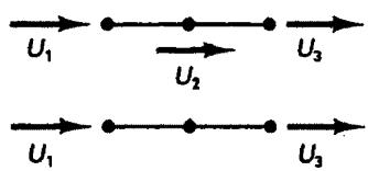
(a) First-level substructure 

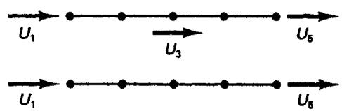
flowchart

```mermaid graph LR A["U1"] --> B["•"] B --> C["•"] C --> D["•"] D --> E["U5"] F["U1"] --> G["•"] G --> H["•"] H --> I["•"] I --> J["U6"] ```

(b) Second-level substructure 

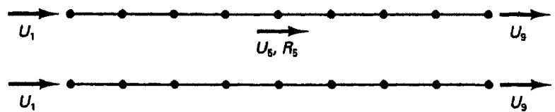
text_image

U₁ U₆, R₅ U₁ U₉

(c) Third-level substructure and actual structure Figure E8.10 Analysis of bar using substructuring to evaluate the equilibrium relations corresponding to $U_{1}$ , $U_{3}$ , and $U_{5}$ : $$ \frac {1 3}{9} \frac {A _ {1} E}{L} \left[ \begin{array}{r r r} 1 & - 1 & 0 \\ - 1 & 3 & - 2 \\ 0 & - 2 & 2 \end{array} \right] \left[ \begin{array}{l} U _ {1} \\ U _ {3} \\ U _ {5} \end{array} \right] = \left[ \begin{array}{c} R _ {1} + \frac {5}{1 2} R _ {2} \\ R _ {3} + \frac {7}{1 2} R _ {2} + \frac {5}{1 2} R _ {4} \\ R _ {5} + \frac {7}{1 2} R _ {4} \end{array} \right] \tag {c} $$ The relation for calculating $U_{4}$ is similar to the one in (b): $$ U _ {4} = \frac {1}{2 4} \left(\frac {3 L}{2 E A _ {1}} R _ {4} + 1 0 U _ {3} + 1 4 U _ {5}\right) $$ Using Gauss elimination on the equations in (c) to condense out $U_{3}$ , we obtain $$ \frac {1 3}{9} \frac {A _ {1} E}{L} \left[ \begin{array}{c c c} \frac {2}{3} & 0 & - \frac {2}{3} \\ - 1 & 3 & - 2 \\ - \frac {2}{3} & 0 & \frac {2}{3} \end{array} \right] \left[ \begin{array}{l} U _ {1} \\ U _ {3} \\ U _ {5} \end{array} \right] = \left[ \begin{array}{c} R _ {1} + \frac {2 2}{3 6} R _ {2} + \frac {1}{3} R _ {3} + \frac {5}{3 6} R _ {4} \\ R _ {3} + \frac {7}{1 2} R _ {2} + \frac {5}{1 2} R _ {4} \\ \frac {1 4}{3 6} R _ {2} + \frac {2}{3} R _ {3} + \frac {3 1}{3 6} R _ {4} + R _ {5} \end{array} \right] $$