Hence, $$ U _ {1} = 1, \quad U _ {2} = 0, \quad U _ {3} = 1, \quad U _ {4} = 0 $$ It should be noted that the rigid body displacement vectors are not unique, but instead the two-dimensional subspace spanned by any two linearly independent rigid body mode vectors is unique. Therefore, any rigid body displacement vector can be written as $$ \left[ \begin{array}{l} U _ {1} \\ U _ {2} \\ U _ {3} \\ U _ {4} \end{array} \right] = \gamma_ {1} \left[ \begin{array}{l} 1 \\ 1 \\ 0 \\ 1 \end{array} \right] + \gamma_ {2} \left[ \begin{array}{l} 1 \\ 0 \\ 1 \\ 0 \end{array} \right] \tag {b} $$ where $\gamma_{1}$ and $\gamma_{2}$ are constants. Note that the rank of K is 2 and the kernel of K is given by the two basis vectors in (b) (see Section 2.3). # 8.2.6 Solution Errors In the preceding sections we presented various algorithms for the solution of KU = R. We applied the solution procedures to some small problems for instructive purposes, but in practical analysis the methods are employed on large systems of equations using a digital computer. It is important to note that the elements of the matrices and the computational results can then be represented to only a fixed number of digits, which introduces errors in the solution. The aim in this section is to discuss the solution errors that can occur in Gauss elimination and to give guidelines for avoiding the introduction of large errors. In order to identify the source of the errors, let us assume that we use a computer in which a number is represented using t digits in single precision. Then, to increase accuracy, double-precision arithmetic may be specified, in which case each number is approximately represented using 2t (or more) digits. As an example, on IBM computers single-precision numbers are represented with 6 digits, whereas double-precision numbers are represented with 16 digits. Considering the finite digit arithmetical operations, the t digits may be used quite differently in different machines. However, most computers, in effect, perform the arithmetic operations and afterward “chop off” all digits beyond the number of digits carried. Therefore, for demonstration purposes we assume in this section that the computer at hand first adds, subtracts, multiplies, and divides two numbers exactly, and then to obtain the finite precision results, chops off all digits beyond the t digits used. In order to demonstrate the finite precision arithmetic, assume that we want to solve the system of equations $$ \left[ \begin{array}{l l} 3. 4 2 5 2 1 & - 3. 4 2 5 2 1 \\ - 3. 4 2 5 2 1 & 1 0 1. 2 4 3 1 \end{array} \right] \left[ \begin{array}{l} U _ {1} \\ U _ {2} \end{array} \right] = \left[ \begin{array}{c} 1. 3 0 2 1 \\ 0. 0 \end{array} \right] \tag {8.44} $$ where K and R are given "exactly." The exact solution is (to 10 digits) $$ U _ {1} = 0. 3 9 3 4 6 3 3 4 4 9; \quad U _ {2} = 0. 0 1 3 3 1 1 4 7 0 9 \tag {8.45} $$ Assume now that for a (hypothetical) computer at hand, t = 3; i.e., each number is represented to only three digits. In this case the solution to the equations in (8.44) would be obtained by first representing K and R using only the first three digits in each number and then calculating the solution by always using only three-digit representations with chopping off of the additional digits. Employing the basic Gauss elimination algorithm (see Sec- tion 8.2.1), the solution would be as follows: $$ \left[ \begin{array}{c c} 3. 4 2 & - 3. 4 2 \\ - 3. 4 2 & 1 0 1 \end{array} \right] \left[ \begin{array}{l} \hat {U} _ {1} \\ \hat {U} _ {2} \end{array} \right] = \left[ \begin{array}{c} 1. 3 0 \\ 0 \end{array} \right] \tag {8.46} $$ where the hats over $U_{1}$ and $U_{2}$ indicate that the solution of (8.46) is different from the solution of (8.44). Using that with chopping to three digits, $$ 1 0 1 - \left(\frac {- 3 . 4 2}{3 . 4 2}\right) (- 3. 4 2) = 1 0 1 - (- 1) (- 3. 4 2) = 9 7. 5 $$ we obtain $\begin{bmatrix} 3.42 & -3.42 \\ 0.0 & 97.5 \end{bmatrix} \begin{bmatrix} \overline{U}_1 \\ \overline{U}_2 \end{bmatrix} = \begin{bmatrix} 1.30 \\ 1.30 \end{bmatrix}$ (8.47) where the bars over $U_{1}$ and $U_{2}$ indicate that we solve (8.46) approximately. Continuing to use three-digit chopping arithmetic, we have $$ \left. \begin{array}{l} \overline {{{U}}} _ {2} = \frac {1 . 3 0}{9 7 . 5} = 0. 0 1 3 3 \\ \overline {{{U}}} _ {1} = \frac {1}{3 . 4 2} [ 1. 3 0 - (- 3. 4 2) (0. 0 1 3 3) ] = \frac {1}{3 . 4 2} (1. 3 4) \\ = 0. 3 9 1 \end{array} \right\} \tag {8.48} $$ Referring to the above example, we can identify two kinds of errors: a truncation error and a round-off error. The truncation error is the error arising because the exact matrix K and load vector R in (8.44) are represented to only three-digit precision, as given in (8.46). The round-off error is the error that arises in the solution of (8.46) because only three-digit arithmetic is used. Considering the situations in which each type of error would be large, we note that the truncation error can be large if the absolute magnitude of the elements in the matrix K including the diagonal elements varies by a large amount. The round-off error can be large if a small diagonal element $d_{ii}$ is used that creates a large multiplier $l_{ij}$ . The reason that the truncation and round-off errors are large under the above conditions is that the basic operation in the factorization is a subtraction of a multiple of the pivot row from the rows below it. If in this operation numbers of widely different magnitudes are subtracted—that have, however, been represented to only a fixed number of digits—the errors in this basic operation can be relatively large. To identify the round-off errors and the truncation errors individually in the example, we need to solve (8.46) exactly, in which case we obtain $$ \left[ \begin{array}{c c} 3. 4 2 & - 3. 4 2 \\ 0 & 9 7. 5 8 \end{array} \right] \left[ \begin{array}{l} \hat {U} _ {1} \\ \hat {U} _ {2} \end{array} \right] = \left[ \begin{array}{l} 1. 3 0 \\ 1. 3 0 \end{array} \right] \tag {8.49} $$ and $\hat{U}_1 = 0.3934393613$ (8.50) $$ \hat {U} _ {2} = 0. 0 1 3 3 2 2 4 0 2 0 $$ The error in the solution arising from initial truncation is therefore $$ \hat {\mathbf {r}} = \left[ \begin{array}{l} U _ {1} \\ U _ {2} \end{array} \right] - \left[ \begin{array}{l} \hat {U} _ {1} \\ \hat {U} _ {2} \end{array} \right] = \left[ \begin{array}{c} 0. 0 0 0 0 2 3 9 8 3 6 \\ - 0. 0 0 0 0 1 0 9 3 1 1 \end{array} \right] \tag {8.51} $$ and the round-off error is $$ \overline {{{\mathbf {r}}}} = \left[ \begin{array}{l} \hat {U} _ {1} \\ \hat {U} _ {2} \end{array} \right] - \left[ \begin{array}{l} \overline {{{U}}} _ {1} \\ \overline {{{U}}} _ {2} \end{array} \right] = \left[ \begin{array}{l} 0. 0 0 2 4 3 9 3 6 1 3 \\ 0. 0 0 0 0 2 2 4 0 2 0 \end{array} \right] \tag {8.52} $$ The total error r is the sum of $\bar{r}$ and $\hat{r}$ , or $$ \mathbf {r} = \left[ \begin{array}{l} U _ {1} \\ U _ {2} \end{array} \right] - \left[ \begin{array}{l} \overline {{U}} _ {1} \\ \overline {{U}} _ {2} \end{array} \right] = \left[ \begin{array}{l} 0. 0 0 2 4 6 3 3 4 4 9 \\ 0. 0 0 0 0 1 1 4 7 0 9 \end{array} \right] \tag {8.53} $$ In this evaluation of the solution errors, we used the exact solutions to (8.44) and (8.49). In practical analyses, these exact solutions cannot be obtained; instead, double-precision arithmetic could be employed to calculate close approximations to them. Consider now that in a specific analysis the solution obtained to the equations $KU = R$ is $\overline{U}$ ; i.e., because of truncation and round-off errors, $\overline{U}$ is calculated instead of U. It appears that the error in the solution can be obtained by evaluating a residual $\Delta R$ , where $$ \Delta \mathbf {R} = \mathbf {R} - \mathbf {K} \overline {{\mathbf {U}}} \tag {8.54} $$ In practice, $\Delta R$ would be calculated using double-precision arithmetic. Substituting KU for R into (8.54), we have for the solution error $r = U - \overline{U}$ , $$ \mathbf {r} = \mathbf {K} ^ {- 1} \Delta \mathbf {R} \tag {8.55} $$ meaning that although $\Delta R$ may be small, the error in the solution may still be large. On the other hand, for an accurate solution $\Delta R$ must be small. Therefore, a small residual $\Delta R$ is a necessary but not a sufficient condition for an accurate solution. EXAMPLE 8.14: Calculate $\Delta R$ and r for the introductory example considered above. Using the values for $\mathbf{R}$ , $\mathbf{K}$ , and $\overline{\mathbf{U}}$ given in (8.44) and (8.48), respectively, we obtain, using (8.54), $$ \boldsymbol {\Delta} \mathbf {R} = \left[ \begin{array}{c} 1. 3 0 2 1 \\ 0 \end{array} \right] - \left[ \begin{array}{c c} 3. 4 2 5 2 1 & - 3. 4 2 5 2 1 \\ - 3. 4 2 5 2 1 & 1 0 1. 2 4 3 1 \end{array} \right] \left[ \begin{array}{c} 0. 3 9 1 \\ 0. 0 1 3 3 \end{array} \right] $$ or $\Delta \mathbf{R} = \left[ \begin{array}{c}0.00839818\\ -0.00042520 \end{array} \right]$ Hence, using (8.55), we have $$ \mathbf {r} = \left[ \begin{array}{l} 0. 0 0 2 5 3 3 3 8 \\ 0. 0 0 0 0 8 1 5 1 \end{array} \right] $$ In this case, $\Delta R$ and r are both relatively small because K is well-conditioned. EXAMPLE 8.15: Consider the system of equations $$ \left[ \begin{array}{c c c c} 4. 8 5 5 & - 4 & 1 & 0 \\ - 4 & 5. 8 5 5 & - 4 & 1 \\ 1 & - 4 & 5. 8 5 5 & - 4 \\ 0 & 1 & - 4 & 4. 8 5 5 \end{array} \right] \left[ \begin{array}{l} U _ {1} \\ U _ {2} \\ U _ {3} \\ U _ {4} \end{array} \right] = \left[ \begin{array}{c} - 1. 5 9 \\ 1 \\ 1 \\ - 1. 6 4 \end{array} \right] $$ Use six-digit arithmetic with chopping to calculate the solution. Following the basic Gauss elimination process, we have $$ \left[ \begin{array}{c c c c} 4. 8 5 5 0 0 & - 4 & 1 & 0 \\ 0 & 2. 5 5 9 4 4 & - 3. 1 7 6 1 0 & 1 \\ 0 & - 3. 1 7 6 1 0 & 5. 6 4 9 0 2 & - 4 \\ 0 & 1 & - 4 & 4. 8 5 5 0 0 \end{array} \right] \left[ \begin{array}{l} \overline {{U}} _ {1} \\ \overline {{U}} _ {2} \\ \overline {{U}} _ {3} \\ \overline {{U}} _ {4} \end{array} \right] = \left[ \begin{array}{l} - 1. 5 9 0 0 0 \\ - 0. 3 0 9 9 8 0 \\ 1. 3 2 7 1 9 \\ - 1. 6 4 0 0 0 \end{array} \right] $$ $$ \left[ \begin{array}{c c c c} 4. 8 5 5 0 0 & - 4 & 1 & 0 \\ 0 & 2. 5 5 9 4 4 & - 3. 1 7 6 1 0 & 1 \\ 0 & 0 & 1. 7 0 7 7 1 & - 2. 7 5 9 0 7 \\ 0 & 0 & - 2. 7 5 9 0 7 & 4. 4 6 4 2 9 \end{array} \right] \left[ \begin{array}{l} \overline {{U}} _ {1} \\ \overline {{U}} _ {2} \\ \overline {{U}} _ {3} \\ \overline {{U}} _ {4} \end{array} \right] = \left[ \begin{array}{l} - 1. 5 9 0 0 0 \\ - 0. 3 0 9 9 8 0 \\ 0. 9 4 2 8 2 7 \\ - 1. 5 1 8 8 8 \end{array} \right] $$ $$ \left[ \begin{array}{c c c c} 4. 8 5 5 0 0 & - 4 & 1 & 0 \\ & 2. 5 5 9 4 4 & - 3. 1 7 6 1 0 & 1 \\ & & 1. 7 0 7 7 1 & - 2. 7 5 9 0 7 \\ & & & 0. 0 0 6 6 0 0 \end{array} \right] \left[ \begin{array}{l} \overline {{U}} _ {1} \\ \overline {{U}} _ {2} \\ \overline {{U}} _ {3} \\ \overline {{U}} _ {4} \end{array} \right] = \left[ \begin{array}{l} - 1. 5 9 0 0 0 \\ - 0. 3 0 9 9 8 0 \\ 0. 9 4 2 8 2 7 \\ 0. 0 0 4 3 9 0 \end{array} \right] $$ The back-substitution yields $\overline{\mathbf{U}} = \begin{bmatrix} 0.686706 \\ 1.63768 \\ 1.62674 \\ 0.665151 \end{bmatrix}$ The exact answer (to seven digits) is $$ \mathbf {U} = \left[ \begin{array}{l} 0. 7 0 3 7 2 4 7 \\ 1. 6 6 5 2 2 5 6 \\ 1. 6 5 4 2 8 3 1 \\ 0. 6 8 2 1 5 6 7 \end{array} \right] $$ Evaluating $\Delta R$ as given in (8.54), we obtain $$ \boldsymbol {\Delta} \mathbf {R} = \left[ \begin{array}{c} - 1. 5 9 \\ 1 \\ 1 \\ - 1. 6 4 \end{array} \right] - \left[ \begin{array}{c} - 1. 5 9 0 0 2 2 3 7 \\ 0. 9 9 9 9 8 3 4 0 \\ 0. 9 9 9 9 4 4 7 0 \\ - 1. 6 3 9 9 7 1 8 9 5 \end{array} \right] = \left[ \begin{array}{c} 0. 0 0 0 0 2 2 3 7 \\ 0. 0 0 0 0 1 6 6 0 \\ 0. 0 0 0 0 5 5 3 0 \\ - 0. 0 0 0 0 2 8 1 0 5 \end{array} \right] $$ Also evaluating $\mathbf{r}$ , we have $\mathbf{r} = \begin{bmatrix} 0.01702 \\ 0.02756 \\ 0.02754 \\ 0.01701 \end{bmatrix}$ We therefore see that $\Delta R$ is relatively much smaller than r. Indeed, the displacement errors are of the order 1 to 2 percent, although the load errors seem to indicate an accurate solution of the equations. Considering (8.55), we must expect that solution accuracy is difficult to obtain when the smallest eigenvalue of K is very small or nearly zero; i.e., the system can almost undergo rigid body motion. Namely, in that case the elements in $K^{-1}$ are large and the solution errors may be large although $\Delta R$ is small. Also, to substantiate this conclusion, we may realize that if $\lambda_{1}$ of K is small, the solution $KU = R$ may be thought of as one step of inverse iteration with a shift close to $\lambda_{1}$ . But the analysis in Section 11.2.1 shows that in such a case the solution tends to have components of the corresponding eigenvector. These components now appear as solution errors. To obtain more information on the solution errors, an analysis can be performed that shows that it is not only a small (near zero) eigenvalue $\lambda_{1}$ but a large ratio of the largest to the smallest eigenvalues of K that determines the solution errors. Namely, in the solution of KU = R, owing to truncation and round-off errors, we may assume that we in fact solve $$ (\mathbf {K} + \delta \mathbf {K}) (\mathbf {U} + \delta \mathbf {U}) = \mathbf {R} \tag {8.56} $$ Assuming that $\delta K \delta U$ is small in relation to the other terms, we have approximately $$ \delta \mathbf {U} = - \mathbf {K} ^ {- 1} \delta \mathbf {K} \mathbf {U} \tag {8.57} $$ or, taking norms, $\frac{\|\delta\mathbf{U}\|}{\|\mathbf{U}\|} \leq \operatorname{cond}(\mathbf{K}) \frac{\|\delta\mathbf{K}\|}{\|\mathbf{K}\|}$ (8.58) where cond(K) is the condition number of K, $$ \operatorname{cond} (\mathbf {K}) = \frac {\lambda_ {n}}{\lambda_ {1}} \tag {8.59} $$ Therefore, a large condition number means that solution errors are more likely. To evaluate an estimate of the solution errors, assume that for a t-digit precision computer, $$ \frac {\| \delta \mathbf {K} \|}{\| \mathbf {K} \|} = 1 0 ^ {- t} \tag {8.60} $$ Also, assuming $s$ -digit precision in the solution, we have $$ \frac {\| \delta \mathbf {U} \|}{\| \mathbf {U} \|} = 1 0 ^ {- s} \tag {8.61} $$ Substituting (8.60) and (8.61) into (8.58), we obtain as an estimate of the number of accurate digits obtained in the solution, $$ s \geq t - \log_ {1 0} [ \operatorname{cond} (\mathbf {K}) ] \tag {8.62} $$ EXAMPLE 8.16: Calculate the condition number of the matrix K used in Example 8.15. Then estimate the accuracy that can be expected in the equation solution. In this case we have $$ \lambda_ {1} = 0. 0 0 0 8 9 8 $$ $$ \lambda_ {4} = 1 2. 9 4 5 2 $$ Hence, $\operatorname{cond}(\mathbf{K}) = 14415.6$ and $\log_{10}[\mathrm{cond}(\mathbf{K})] = 4.15883$ Thus the number of accurate digits using six-digit arithmetic predicted using (8.62) is $$ s \geq 6 - 4. 1 6 $$ or one- to two-digit accuracy can be expected. Comparing this result with the results obtained in Example 8.15, we observe that, indeed, only one- to two-digit accuracy was obtained. The condition number of K can in practice be evaluated approximately by calculating an upper bound for $\lambda_{n}$ , say $\lambda_{n}^{\mu}$ , $$ \lambda_ {n} ^ {u} = \left\| \mathbf {K} \right\| \tag {8.63} $$ where any matrix norm may be used (see Example 8.17), and evaluating a lower bound for $\lambda_{1}$ , say $\lambda_{1}^{l}$ , using inverse iteration (see Section 11.2.1). We thus have $$ \operatorname{cond} (\mathbf {K}) \doteq \frac {\lambda_ {n} ^ {u}}{\lambda_ {1} ^ {l}} \tag {8.64} $$ EXAMPLE 8.17: Calculate an estimate of the condition number of the matrix K used in Example 8.15. Here we have, using the $\infty$ norm (see Section 2.7), $$ \| \mathbf {K} \| _ {\infty} = 1 4. 8 5 5 $$ and by inverse iteration we obtain $\lambda_{1} = 0.0009$ . Hence, $$ \log_ {1 0} (\text { cond } (\mathbf {K})) = 4. 2 1 7 6 $$ and the conclusions reached in Example 8.16 are still valid. The preceding considerations on round-off and truncation errors yield the following two important results: 1. Both types of errors can be expected to be large if structures with widely varying stiffness are analyzed. Large stiffness differences may be due to different material moduli, or they may be the result of the finite element modeling used, in which case a more effective model can frequently be chosen. This may be achieved by the use of finite elements that are nearly equal in size and have almost the same lengths in each dimension, the use of master-slave degrees of freedom, i.e., constraint equations (see Section 4.2.2 and Example 8.19), and relative degrees of freedom (see Example 8.20). 2. Since truncation errors are most significant, to improve the solution accuracy it is necessary to evaluate both the stiffness matrix K and the solution of KU = R in double precision. It is not sufficient (a) to evaluate K in single precision and then solve the equations in double precision (see Example 8.18), or (b) to evaluate K in single precision, solve the equations in single precision using a Gauss elimination procedure, and then iterate for an improvement in the solution employing, for example, the Gauss-Seidel method. We demonstrate these two conclusions by means of some simple examples. 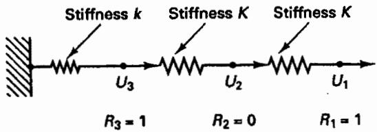EXAMPLE 8.18: Consider the simple spring system in Fig. E8.18. Calculate the displacements when $k = 1$ , $K = 10,000$ using four-digit arithmetic. The equilibrium equations of the system are $$ \left[ \begin{array}{c c c} K & - K & 0 \\ - K & 2 K & - K \\ 0 & - K & K + k \end{array} \right] \left[ \begin{array}{l} U _ {1} \\ U _ {2} \\ U _ {3} \end{array} \right] = \left[ \begin{array}{l} 1 \\ 0 \\ 1 \end{array} \right] $$ 

text_image

Stiffness k Stiffness K Stiffness K U₃ U₂ U₁ R₃ = 1 R₂ = 0 R₁ = 1

Figure E8.18 Simple spring system Substituting $K = 10,000$ , $k = 1$ and using four-digit arithmetic, we have $$ \left[ \begin{array}{c c c} 1 0, 0 0 0 & - 1 0, 0 0 0 & 0 \\ - 1 0, 0 0 0 & 2 0, 0 0 0 & - 1 0, 0 0 0 \\ 0 & - 1 0, 0 0 0 & 1 0, 0 0 0 \end{array} \right] \left[ \begin{array}{l} U _ {1} \\ U _ {2} \\ U _ {3} \end{array} \right] = \left[ \begin{array}{l} 1 \\ 0 \\ 1 \end{array} \right] $$ The triangularization of the coefficient matrix gives $$ \left[ \begin{array}{c c c} 1 0, 0 0 0 & - 1 0, 0 0 0 & 0 \\ 0 & 1 0, 0 0 0 & - 1 0, 0 0 0 \\ 0 & 0 & 0 \end{array} \right] \left[ \begin{array}{l} U _ {1} \\ U _ {2} \\ U _ {3} \end{array} \right] = \left[ \begin{array}{l} 1. 0 \\ 1. 0 \\ 2. 0 \end{array} \right] $$ Hence, a solution is not possible, because $d_{nn} = 0.0$ . To obtain a solution we may employ higher-digit arithmetic. In practice, this would mean that double-precision arithmetic would be used, i.e., in this case, eight- instead of four-digit arithmetic. Using eight-digit arithmetic (indeed five digits would be sufficient), we obtain the exact solution as follows: $$ \begin{array}{l} \left[ \begin{array}{c c c} 1 0, 0 0 0 & - 1 0, 0 0 0 & 0 \\ - 1 0, 0 0 0 & 2 0, 0 0 0 & - 1 0, 0 0 0 \\ 0 & - 1 0, 0 0 0 & 1 0, 0 0 1 \end{array} \right] \left[ \begin{array}{l} U _ {1} \\ U _ {2} \\ U _ {3} \end{array} \right] = \left[ \begin{array}{l} 1 \\ 0 \\ 1 \end{array} \right] \\ \left[ \begin{array}{c c c} 1 0, 0 0 0 & - 1 0, 0 0 0 & 0 \\ 0 & 1 0, 0 0 0 & - 1 0, 0 0 0 \\ 0 & 0 & 1 \end{array} \right] \left[ \begin{array}{l} U _ {1} \\ U _ {2} \\ U _ {3} \end{array} \right] = \left[ \begin{array}{l} 1. 0 \\ 1. 0 \\ 2. 0 \end{array} \right] \\ \end{array} $$ Hence, $\mathbf{U} = \begin{bmatrix} 2.0002\\ 2.0001\\ 2.0 \end{bmatrix}$ This example shows that a sufficient number of digits carried in the arithmetic may be vital for the solution not to break down. EXAMPLE 8.19: Use the master-slave solution procedure to analyze the system considered in Fig. E8.18. The basic assumption in the master-slave analysis is the use of the constraint equations $$ U _ {1} = U _ {2} = U _ {3} $$ The equilibrium equation governing the system is thus $$ k U _ {1} = 2 $$ Substituting for $k$ , we obtain $U_{1} = 2$ and the complete solution is $$ \mathbf {U} = \left[ \begin{array}{l} 2. 0 \\ 2. 0 \\ 2. 0 \end{array} \right] $$ This solution is approximate. However, comparing the solution with the exact result (see Example 8.18), we find that the main response is properly predicted. EXAMPLE 8.20: Use relative degrees of freedom to analyze the system in Fig. E8.18. Using relative degrees of freedom, the displacement degrees of freedom defined are $U_{3}$ , $\Delta_{1}$ , and $\Delta_{2}$ , where $$ U _ {2} = U _ {3} + \Delta_ {2} $$ $$ U _ {1} = U _ {2} + \Delta_ {1} $$ or we have $$ \left[ \begin{array}{l} U _ {1} \\ U _ {2} \\ U _ {3} \end{array} \right] = \left[ \begin{array}{l l l} 1 & 1 & 1 \\ 0 & 1 & 1 \\ 0 & 0 & 1 \end{array} \right] \left[ \begin{array}{l} \Delta_ {1} \\ \Delta_ {2} \\ U _ {3} \end{array} \right] \tag {a} $$ The matrix relating the degrees of freedom $\Delta_{1}$ , $\Delta_{2}$ , and $U_{3}$ to the degrees of freedom $U_{1}$ , $U_{2}$ , and $U_{3}$ is the matrix T. The equilibrium equations for the system using relative degrees of freedom are $(\mathbf{T}^{T}\mathbf{K}\mathbf{T})\mathbf{U}_{\mathrm{rel}} = \mathbf{T}^{T}\mathbf{R}$ ; i.e., the equilibrium equations are now $$ \left[ \begin{array}{c c c} 1 0, 0 0 0 & 0 & 0 \\ 0 & 1 0, 0 0 0 & 0 \\ 0 & 0 & 1. 0 \end{array} \right] \left[ \begin{array}{l} \Delta_ {1} \\ \Delta_ {2} \\ U _ {3} \end{array} \right] = \left[ \begin{array}{l} 1. 0 \\ 1. 0 \\ 2. 0 \end{array} \right] \tag {b} $$ with the solution $$ \Delta_ {1} = 0. 0 0 0 1 $$ $$ \Delta_ {2} = 0. 0 0 0 1 $$ $$ U _ {3} = 2. 0 $$ Hence, we obtain $$ U _ {1} = 2. 0 0 0 2 $$ $$ U _ {2} = 2. 0 0 0 1 $$ $$ U _ {3} = 2. 0 0 0 0 $$ Therefore, using four-digit arithmetic, we obtain the exact solution of the system if relative degrees of freedom are used (see Example 8.18). However, it should be noted that the equilibrium equations corresponding to the relative degrees of freedom would have to be formed directly, i.e., without the transformation used in this example. # 8.2.7 Exercises 8.1. Consider the cantilever beam in Example 8.1 with the given stiffness matrix. Calculate the experimental results that you expect to obtain in a laboratory experiment for the stiffnesses of the beam, as described in Figs. 8.3 to 8.6 for the simply supported beam discussed in the text. That is, give the forces in the clamps and the deflected shapes of the cantilever beam corresponding to the stiffness measurements of the four cases: all four clamps present, clamp 1 removed, clamps 1 and 2 removed, and clamps 1, 2, and 3 removed. 8.2. Given the stiffness matrix of the cantilever beam in Example 8.1, calculate the stiffness matrix corresponding to $U_{2}$ and $U_{4}$ only, that is, with the degrees of freedom $U_{1}$ and $U_{3}$ released. Then calculate and plot the deflected shapes of the beam described by $U_{2}$ and $U_{4}$ only when $U_{2} = 1$ , $U_{4} = 0$ and when $U_{2} = 0$ , $U_{4} = 1$ . 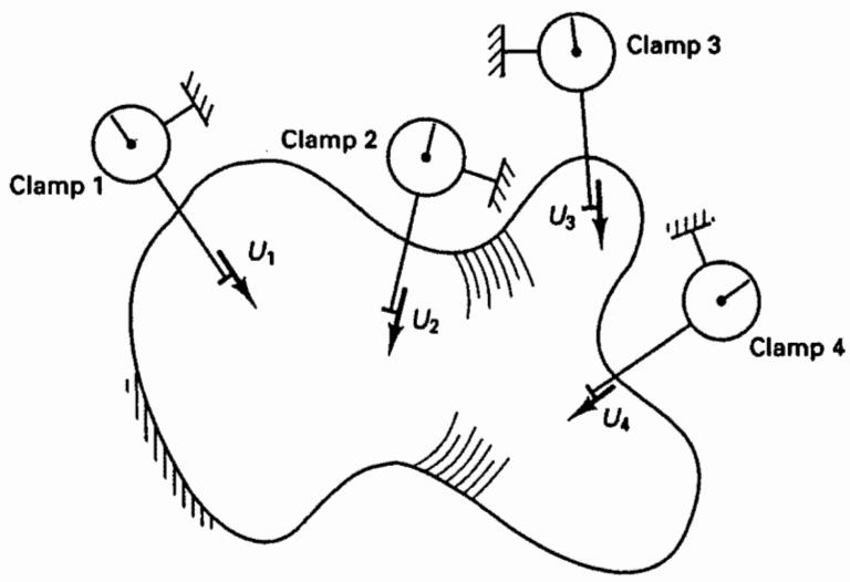8.3. A laboratory experiment is performed to obtain the stiffness matrix of a structure. The clamps shown are used, and the following $4 \times 4$ stiffness matrix is measured: $$ \mathbf {K} = \left[ \begin{array}{c c c c} 1 4 & - 6 & 1 & 0 \\ - 6 & 1 4 & - 7 & 1 \\ 1 & - 7 & 1 6 & - 8 \\ 0 & 1 & - 8 & 1 8 \end{array} \right] $$ 

flowchart

```mermaid graph TD Clamp1["Clamp 1"] --> U1["U1"] Clamp2["Clamp 2"] --> U2["U2"] Clamp3["Clamp 3"] --> U3["U3"] Clamp4["Clamp 4"] --> U4["U4"] U1 --> U2 U2 --> U3 U3 --> U4 ```

All clamps are firmly attached to structure Clamp 2 is then removed, and the following $3 \times 3$ stiffness matrix is measured: $$ \tilde {\mathbf {K}} = \left[ \begin{array}{c c c} \frac {8 0}{7} & - 2 & \frac {3}{7} \\ - 2 & \frac {2 5}{2} & - \frac {1 5}{2} \\ \frac {3}{7} & - \frac {1 5}{2} & 1 7 \end{array} \right] $$ While you are sure that the matrix K has been correctly established, there is some doubt as to whether the matrix $\tilde{K}$ has been measured correctly because clamp 3 might not have worked properly. Check whether the stiffness elements in $\tilde{K}$ are correct, and if there is an error, give the details of the error. 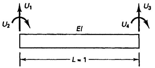8.4. The stiffness matrix of the beam element shown in (a) is given as $$ \mathbf {K} = E I \left[ \begin{array}{c c c c} U _ {1} & U _ {2} & U _ {3} & U _ {4} \\ 1 2 & - 6 & - 1 2 & - 6 \\ - 6 & 4 & 6 & 2 \\ - 1 2 & 6 & 1 2 & 6 \\ - 6 & 2 & 6 & 4 \end{array} \right] $$ Calculate the stiffness of the element assemblage in (b) corresponding to the degree of freedom $\theta$ only. 

text_image

U₁ U₂ EI U₄ U₃ L = 1

(a) 

text_image

L = 1 L = 1 EI Roller θ M 2EI

$$ M = k _ {1 1} \theta ; k _ {1 1} = ? $$ (b) 8.5. The cantilever beam in Example 8.1 is loaded with a concentrated force corresponding to $U_{2}$ ; hence, the governing equations are $$ \left[ \begin{array}{r r r r} 7 & - 4 & 1 & 0 \\ - 4 & 6 & - 4 & 1 \\ 1 & - 4 & 5 & - 2 \\ 0 & 1 & - 2 & 1 \end{array} \right] \left[ \begin{array}{l} U _ {1} \\ U _ {2} \\ U _ {3} \\ U _ {4} \end{array} \right] = \left[ \begin{array}{l} 0 \\ 1 \\ 0 \\ 0 \end{array} \right] $$ Calculate the displacement solution by performing Gauss elimination on the displacement variables in the order $U_{4}$ , $U_{3}$ , and $U_{1}$ . 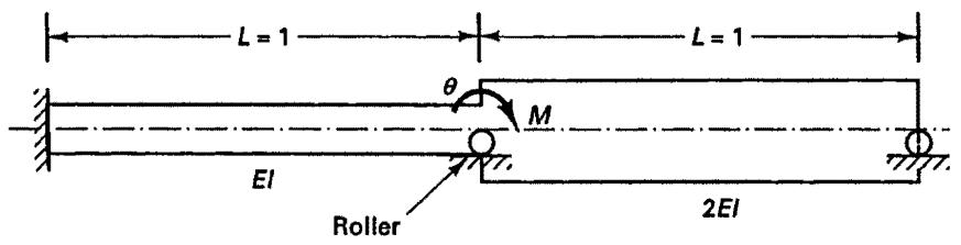8.6. Consider the four-node finite element shown with its boundary conditions. Assume that Gauss elimination is performed in the usual order for $U_{1}, U_{2}, \ldots$ , and so on, i.e., from the lowest to the highest degree of freedom number. Determine for cases 1 to 3 whether any zero diagonal element will be encountered in the elimination process, and if so, at what stage of the solution this will be the case. 

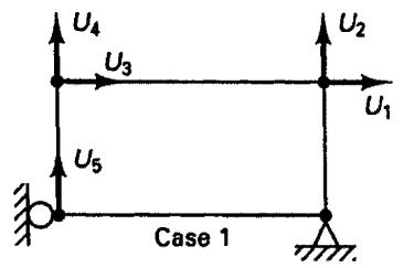
text_image

U₄ U₃ U₂ U₁ U₅ Case 1


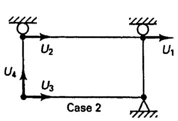
text_image

U2 U4 U3 Case 2 U1


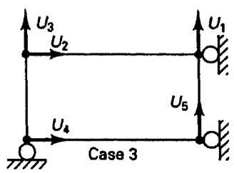
text_image

U₃ U₂ U₁ U₄ U₅ Case 3

8.7. Establish the LDL $^{T}$ factorization of the cantilever beam stiffness matrix K in Example 8.1 (K is the result of the first experiment; see Exercise 8.5). Use this factorization to calculate det K and to calculate the Cholesky factor L of K. 8.8. Prove that corresponding to (8.10) and (8.14) we indeed have $\mathbf{S} = \mathbf{D}\tilde{\mathbf{S}}$ and $\tilde{\mathbf{S}} = \mathbf{L}^T$ .