The initial conditions are
$$
{ } ^ { 0 } U _ { 1 } = { } ^ { 0 } \dot { U } _ { 1 } = { } ^ { 0 } \ddot { U } _ { 1 } = { } ^ { 0 } U _ { 2 } = { } ^ { 0 } \dot { U } _ { 2 } = 0 ; \quad { } ^ { 0 } \ddot { U } _ { 2 } = 1 0
$$
Hence, using (9.7) to obtain the starting value $-\Delta t U_1$ , we obtain $-\Delta t U_1 = 0$ .
We can now use, for each time step, (a) and (c) to solve for $t^{+\Delta t}U_1$ and then (b) and (d) to solve for $t^{+\Delta t}U_2$ . We should note that in this solution we evaluate $t^{+\Delta t}U_1$ by projecting ahead from the equilibrium configuration at time $t$ of the degree of freedom 1, and we then accept this value of $t^{+\Delta t}U_1$ to evaluate $t^{+\Delta t}U_2$ implicitly. Using this procedure we obtain with $\Delta t = 0.28$ the following data:
| Time | $\Delta t$ | $2\Delta t$ | $3\Delta t$ | $4\Delta t$ | $5\Delta t$ | $6\Delta t$ | $7\Delta t$ | $8\Delta t$ | $9\Delta t$ | $10\Delta t$ | $11\Delta t$ | $12\Delta t$ |
| $^{1}U$ | 0.0 | 0.0285 | 0.156 | 0.457 | 0.962 | 1.63 | 2.33 | 2.88 | 3.11 | 2.90 | 2.24 | 1.25 |
| 0.364 | 1.35 | 2.68 | 3.98 | 4.93 | 5.32 | 5.12 | 4.50 | 3.70 | 2.99 | 2.54 | 2.39 |
This solution compares with the response calculated in Example 9.1. If, however, we now try to obtain a solution with $\Delta t = 28$ , we find that the solution is unstable; i.e., the predicted displacements very rapidly grow out of bound.
While here explicit and implicit integrations are combined, in an alternative solution approach, a single implicit time integration scheme is used for the complete domain, but the stiffness of the very flexible part is not added to the coefficient matrix, and dynamic equilibrium is satisfied by iteration (see, for example, K. J. Bathe and V. Sonnad [A] and Section 8.3.2). Finally, it may also be effective to switch between explicit and implicit integrations during the complete response solution.
# 9.2.6 Exercises
9.1. Consider the two degree of freedom system
$$
\left[ \begin{array}{l l} 1 & 0 \\ 0 & 2 \end{array} \right] \left[ \begin{array}{l} \ddot {U} _ {1} \\ \ddot {U} _ {2} \end{array} \right] + \left[ \begin{array}{c c} 8 & - 3 \\ - 3 & 4 \end{array} \right] \left[ \begin{array}{l} U _ {1} \\ U _ {2} \end{array} \right] = \left[ \begin{array}{l} 1 0 \\ 0 \end{array} \right]
$$
with the initial conditions ${}^{0}U = {}^{0}\dot{U} = 0$ . Use the central difference method to calculate the response of the system to a reasonable accuracy for time 0 to time 4.
9.2. Consider the same system equations as in Exercise 9.1 but use the trapezoidal rule to calculate the system response.
9.3. Develop a computational scheme for which the Wilson $\theta$ method and the trapezoidal rule are special cases. Give the computational scheme in tabular form (as Table 9.3 for the Newmark method). See E.L. Wilson, I. Farhoomand and K.J. Bathe [A].
9.4. Show that when using as the first substep $(2-\sqrt{2})\Delta t$ in the Bathe method, the two coefficient matrices (used in Table 9.4) are identical.
9.5. Consider the single degree of freedom equation
$$
2 \ddot {U} + 4 U = 0; \quad {} ^ {0} U = 1 0 ^ {- 1 2}; \quad {} ^ {0} \dot {U} = 0
$$
(which is obtained by setting $U_{1} = 0$ in the system in Exercise 9.1).
Assume that the time step used in the time integration is $1.01 \times \Delta t_{cr}$ . Estimate after how many time steps the solution will reach overflow (which is, for the computer used, given by $10^{30}$ ).
9.6. Solve the equations given in Exercise 9.1 by using the central difference method for the time integration of $U_{1}$ and the trapezoidal rule for the time integration of $U_{2}$ .
# 9.3 MODE SUPERPOSITION
Tables 9.2 to 9.4, summarizing the implicit direct integration schemes, show that if a diagonal mass matrix and no damping are assumed, the number of operations for one time step are—as a rough estimate—somewhat larger than $2nm_{K}$ , where n and $m_{K}$ are the order and half-bandwidth of the stiffness matrix considered, respectively (assuming constant column heights or a mean half-bandwidth, see Section 8.2.3). The $2nm_{K}$ operations are required for the solution of the system equations in each time step. The initial triangular factorization of the effective stiffness matrix requires additional operations. Furthermore, if a consistent mass matrix is used or a damping matrix is included in the analysis, an additional number of operations proportional to $nm_{K}$ is required per time step. Therefore, neglecting the operations for the initial calculations, a total number of about $\alpha nm_{K}s$ operations is required in the complete integration, where $\alpha$ depends on the characteristics of the matrices used and s is the number of time steps.
Using the central difference method, the number of operations per step is usually much less (for the reasons given in Section 9.2.1).
These considerations show that the number of operations required in a direct integration solution are directly proportional to the number of time steps and that the use of implicit direct integration can be expected to be effective only when the response for a relatively short duration (i.e., for not too many time steps) is required. If the integration must be carried out for many time steps, it may be more effective to first transform the equilibrium equations (9.1) into a form in which the step-by-step solution is less costly. In particular, since the number of operations required is directly proportional to the half-bandwidth $m_{K}$ of the stiffness matrix, a reduction in $m_{K}$ would decrease proportionally the cost of the step-by-step solution.
It is important at this stage to fully recognize what we have proposed to pursue. We recall that $(9.1)$ are the equilibrium equations obtained when the finite element interpolation functions are used in the evaluation of the virtual work equation $(4.7)$ (see Section 4.2.1). The resulting matrices K, M, and C have a bandwidth that is determined by the numbering of the finite element nodal points. Therefore, the topology of the finite element mesh determines the order and bandwidth of the system matrices. In order to reduce the bandwidth of the system matrices, we may rearrange the nodal point numbering; however, there is a limit on the minimum bandwidth that can be obtained in this way, and we therefore set out to follow a different procedure.
# 9.3.1 Change of Basis to Modal Generalized Displacements
We propose to transform the equilibrium equations into a more effective form for direct integration by using the following transformation on the n finite element nodal point displacements in U,
$$
\mathbf {U} (t) = \mathbf {P X} (t) \tag {9.30}
$$
where $\mathbf{P}$ is an $n \times n$ square matrix and $\mathbf{X}(t)$ is a time-dependent vector of order $n$ . The
transformation matrix P is still unknown and will have to be determined. The components of X are referred to as generalized displacements. Substituting (9.30) into (9.1) and premultiplying by $P^{T}$ , we obtain
$$
\tilde {\mathbf {M}} \ddot {\mathbf {X}} (t) + \tilde {\mathbf {C}} \dot {\mathbf {X}} (t) + \tilde {\mathbf {K}} \mathbf {X} (t) = \tilde {\mathbf {R}} (t) \tag {9.31}
$$
where $\tilde{\mathbf{M}} = \mathbf{P}^T\mathbf{M}\mathbf{P};\qquad \tilde{\mathbf{C}} = \mathbf{P}^T\mathbf{C}\mathbf{P};\qquad \tilde{\mathbf{K}} = \mathbf{P}^T\mathbf{K}\mathbf{P};\qquad \tilde{\mathbf{R}} = \mathbf{P}^T\mathbf{R}$ (9.32)
It should be noted that this transformation is obtained by substituting (9.30) into (4.8) to express the element displacements in terms of the generalized displacements,
$$
\mathbf {u} ^ {(m)} (x, y, z, t) = \mathbf {H} ^ {(m)} \mathbf {P} \mathbf {X} (t) \tag {9.33}
$$
and then using (9.33) in the virtual work equation (4.7). Therefore, in essence, to obtain (9.31) from (9.1), a change of basis from the finite element displacement basis to a generalized displacement basis has been performed (see Section 2.5).
The objective of the transformation is to obtain new system stiffness, mass, and damping matrices $\tilde{K}$ , $\tilde{M}$ , and $\tilde{C}$ , which have a smaller bandwidth than the original system matrices, and the transformation matrix P should be selected accordingly. In addition, it should be noted that P must be nonsingular (i.e., the rank of P must be n) in order to have a unique relation between any vectors U and X as expressed in (9.30).
In theory, there can be many different transformation matrices P, which would reduce the bandwidth of the system matrices. However, in practice, an effective transformation matrix is established using the displacement solutions of the free-vibration equilibrium equations with damping neglected,
$$
\mathbf {M} \ddot {\mathbf {U}} + \mathbf {K} \mathbf {U} = \mathbf {0} \tag {9.34}
$$
The solution to (9.34) can be postulated to be of the form
$$
\mathbf {U} = \boldsymbol {\phi} \sin \omega (t - t _ {0}) \tag {9.35}
$$
where $\phi$ is a vector of order n, t is the time variable, $t_{0}$ is a time constant, and $\omega$ is a constant identified to represent the frequency of vibration (radians/second) of the vector $\phi$ .
Substituting (9.35) into (9.34), we obtain the generalized eigenproblem, from which $\phi$ and $\omega$ must be determined,
$$
\mathbf {K} \boldsymbol {\phi} = \omega^ {2} \mathbf {M} \boldsymbol {\phi} \tag {9.36}
$$
The eigenproblem in (9.36) yields the $n$ eigensolutions $(\omega_1^2, \phi_1), (\omega_2^2, \phi_2), \ldots, (\omega_n^2, \phi_n)$ , where the eigenvectors are $\mathbf{M}$ -orthonormalized (see Section 10.2.1); i.e.,
$$
\boldsymbol {\phi} _ {i} ^ {T} \mathbf {M} \boldsymbol {\phi} _ {j} \left\{ \begin{array}{l l} = 1; & i = j \\ = 0; & i \neq j \end{array} \right. \tag {9.37}
$$
and $0 \leq \omega_{1}^{2} \leq \omega_{2}^{2} \leq \omega_{3}^{2} \leq \dots \leq \omega_{n}^{2}$ (9.38)
The vector $\phi_{i}$ is called the ith-mode shape vector, and $\omega_{i}$ is the corresponding frequency of vibration (radians/second). It should be emphasized that (9.34) is satisfied using any of the n displacement solutions $\phi_{i}\sin\omega_{i}(t-t_{0}), i=1,2,\ldots,n$ . For a physical interpretation of $\omega_{i}$ and $\phi_{i}$ , see Example 9.6 and Exercise 9.8.
Defining a matrix $\Phi$ whose columns are the eigenvectors $\phi_{i}$ and a diagonal matrix $\Omega^{2}$ , which stores the eigenvalues $\omega_{i}^{2}$ on its diagonal; i.e.,
$$
\boldsymbol {\Phi} = [ \boldsymbol {\Phi} _ {1}, \boldsymbol {\Phi} _ {2}, \dots , \boldsymbol {\Phi} _ {n} ]; \quad \boldsymbol {\Omega} ^ {2} = \left[ \begin{array}{c c c c c} \omega_ {1} ^ {2} & & & & \\ & \omega_ {2} ^ {2} & & & \\ & & \ddots & & \\ & & & \ddots & \\ & & & & \omega_ {n} ^ {2} \end{array} \right] \tag {9.39}
$$
we can write the $n$ solutions to (9.36) as
$$
\mathbf {K} \boldsymbol {\Phi} = \mathbf {M} \boldsymbol {\Phi} \boldsymbol {\Omega} ^ {2} \tag {9.40}
$$
Since the eigenvectors are M-orthonormal, we have
$$
\boldsymbol {\Phi} ^ {T} \mathbf {K} \boldsymbol {\Phi} = \boldsymbol {\Omega} ^ {2}; \quad \boldsymbol {\Phi} ^ {T} \mathbf {M} \boldsymbol {\Phi} = \mathbf {I} \tag {9.41}
$$
It is now apparent that the matrix $\Phi$ would be a suitable transformation matrix $\mathbf{P}$ in (9.30). Using
$$
\mathbf {U} (t) = \boldsymbol {\Phi} \mathbf {X} (t) \tag {9.42}
$$
we obtain equilibrium equations that correspond to the modal generalized displacements
$$
\ddot {\mathbf {X}} (t) + \boldsymbol {\Phi} ^ {T} \mathbf {C} \boldsymbol {\Phi} \dot {\mathbf {X}} (t) + \boldsymbol {\Omega} ^ {2} \mathbf {X} (t) = \boldsymbol {\Phi} ^ {T} \mathbf {R} (t) \tag {9.43}
$$
The initial conditions on $\mathbf{X}(t)$ are obtained using (9.42) and the M-orthonormality of $\Phi$ ; i.e., at time 0 we have
$$
{ } ^ { 0 } \mathbf { X } = \mathbf { \Phi } ^ { T } \mathbf { M } { } ^ { 0 } \mathbf { U } ; \quad { } ^ { 0 } \dot { \mathbf { X } } = \mathbf { \Phi } ^ { T } \mathbf { M } { } ^ { 0 } \dot { \mathbf { U } } \tag {9.44}
$$
The equations in (9.43) show that if a damping matrix is not included in the analysis, the finite element equilibrium equations are decoupled when using in the transformation matrix P the free-vibration mode shapes of the finite element system. Since the derivation of the damping matrix can in many cases not be carried out explicitly and the damping effects can be included only approximately, it is reasonable to use a damping matrix that includes all required effects but at the same time allows an effective solution of the equilibrium equations. In many analyses damping effects are neglected altogether, and it is this case that we shall discuss first, see also J.W. Tedesco, W.G. McDougal, and C.A. Ross [A].
EXAMPLE 9.6: Calculate the transformation matrix $\Phi$ for the problem considered in Examples 9.1 to 9.4 and thus establish the decoupled equations of equilibrium in the basis of mode shape vectors.
For the system under consideration we have
$$
\mathbf {K} = \left[ \begin{array}{c c} 6 & - 2 \\ - 2 & 4 \end{array} \right]; \quad \mathbf {M} = \left[ \begin{array}{c c} 2 & 0 \\ 0 & 1 \end{array} \right]; \quad \mathbf {R} = \left[ \begin{array}{c} 0 \\ 1 0 \end{array} \right]
$$
The generalized eigenproblem to be solved is therefore
$$
\left[ \begin{array}{c c} 6 & - 2 \\ - 2 & 4 \end{array} \right] \boldsymbol {\phi} = \omega^ {2} \left[ \begin{array}{c c} 2 & 0 \\ 0 & 1 \end{array} \right] \boldsymbol {\phi}
$$
The solution is obtained by one of the methods given in Chapters 10 and 11. Here we simply give
the two solutions without derivations:
$$
\begin{array}{l} \omega_ {1} ^ {2} = 2; \quad \phi_ {1} = \left[ \begin{array}{c} \frac {1}{\sqrt {3}} \\ \frac {1}{\sqrt {3}} \end{array} \right] \\ \omega_ {2} ^ {2} = 5; \quad \phi_ {2} = \left[ \begin{array}{l} \frac {1}{2} \sqrt {\frac {2}{3}} \\ - \sqrt {\frac {2}{3}} \end{array} \right] \\ \end{array}
$$
Therefore, considering the free-vibration equilibrium equations of the system
$$
\left[ \begin{array}{l l} 2 & 0 \\ 0 & 1 \end{array} \right] \ddot {\mathbf {U}} (t) + \left[ \begin{array}{c c} 6 & - 2 \\ - 2 & 4 \end{array} \right] \mathbf {U} (t) = \mathbf {0} \tag {a}
$$
the following two solutions are possible:
$$
\mathbf {U} _ {1} (t) = \left[ \begin{array}{c} \frac {1}{\sqrt {3}} \\ \frac {1}{\sqrt {3}} \end{array} \right] \sin \sqrt {2} (t - t _ {0} ^ {1}) \quad \text { and } \quad \mathbf {U} _ {2} (t) = \left[ \begin{array}{c} \frac {1}{2} \sqrt {\frac {2}{3}} \\ - \sqrt {\frac {2}{3}} \end{array} \right] \sin \sqrt {5} (t - t _ {0} ^ {2})
$$
That the vectors $\mathbf{U}_1(t)$ and $\mathbf{U}_2(t)$ indeed satisfy the relation in (a) can be verified simply by substituting $\mathbf{U}_1$ and $\mathbf{U}_2$ into the equilibrium equations. The actual solution to the equations in (a) is of the form
$$
\mathbf {U} (t) = \alpha \left[ \begin{array}{c} \frac {1}{\sqrt {3}} \\ \frac {1}{\sqrt {3}} \end{array} \right] \sin \sqrt {2} (t - t _ {0} ^ {1}) + \beta \left[ \begin{array}{c} \frac {1}{2} \sqrt {\frac {2}{3}} \\ - \sqrt {\frac {2}{3}} \end{array} \right] \sin \sqrt {5} (t - t _ {0} ^ {2})
$$
where $\alpha$ , $\beta$ , $t_{0}^{1}$ , and $t_{0}^{2}$ are determined by the initial conditions on U and $\dot{U}$ . In particular, if we impose initial conditions corresponding to $\alpha$ (or $\beta$ ) only, we find that the system vibrates in the corresponding eigenvector with frequency $\sqrt{2}$ rad/sec (or $\sqrt{5}$ rad/sec). The general procedure of solution for $\alpha$ , $\beta$ , $t_{1}^{0}$ , and $t_{2}^{0}$ is discussed in Section 9.3.2.
Having evaluated $(\omega_{1}^{2}, \phi_{1})$ and $(\omega_{2}^{2}, \phi_{2})$ for the problem in Examples 9.1 to 9.4, we arrive at the following equilibrium equations in the basis of eigenvectors:
$$
\ddot {\mathbf {X}} (t) + \left[ \begin{array}{l l} 2 & 0 \\ 0 & 5 \end{array} \right] \mathbf {X} (t) = \left[ \begin{array}{c c} \frac {1}{\sqrt {3}} & \frac {1}{\sqrt {3}} \\ \frac {1}{2} \sqrt {\frac {2}{3}} & - \sqrt {\frac {2}{3}} \end{array} \right] \left[ \begin{array}{l} 0 \\ 1 0 \end{array} \right]
$$
$$
\mathbf {X} (t) + \left[ \begin{array}{l l} 2 & 0 \\ 0 & 5 \end{array} \right] \mathbf {X} (t) = \left[ \begin{array}{c} \frac {1 0}{\sqrt {3}} \\ - 1 0 \sqrt {\frac {2}{3}} \end{array} \right] \tag {or}
$$
# 9.3.2 Analysis with Damping Neglected
If velocity-dependent damping effects are not included in the analysis, (9.43) reduces to
$$
\ddot {\mathbf {X}} (t) + \boldsymbol {\Omega} ^ {2} \mathbf {X} (t) = \boldsymbol {\Phi} ^ {T} \mathbf {R} (t) \tag {9.45}
$$
i.e., $n$ individual equations of the form
$$
\left. \begin{array}{r l} \ddot {x} _ {i} (t) + \omega_ {i} ^ {2} x _ {i} (t) & = r _ {i} (t) \\ r _ {i} (t) & = \boldsymbol {\phi} _ {i} ^ {T} \mathbf {R} (t) \end{array} \right\} \quad i = 1, 2, \dots , n \tag {9.46}
$$
with $x_{i}\big|_{t = 0} = \phi_{i}^{T}\mathbf{M}^{0}\mathbf{U}$
$$
\dot {x} _ {i} \big | _ {t = 0} = \boldsymbol {\Phi} _ {i} ^ {T} \mathbf {M} ^ {0} \dot {\mathbf {U}}
$$
We note that the ith typical equation in (9.46) is the equilibrium equation of a single degree of freedom system with unit mass and stiffness $\omega_{i}^{2}$ and initial conditions established from (9.44). The solution to each equation in (9.46) can be obtained using the integration algorithms in Tables 9.1 to 9.4 or can be calculated using the Duhamel integral:
$$
x _ {i} (t) = \frac {1}{\omega_ {i}} \int_ {0} ^ {t} r _ {i} (\tau) \sin \omega_ {i} (t - \tau) d \tau + \alpha_ {i} \sin \omega_ {i} t + \beta_ {i} \cos \omega_ {i} t \tag {9.47}
$$
where $\alpha_{i}$ and $\beta_{i}$ are determined from the initial conditions in (9.46). The Duhamel integral in (9.47) may have to be evaluated numerically. In addition, it should be noted that various other integration methods could also be used in the solution of (9.46).
For the complete response, the solution to all n equations in (9.46), $i = 1, 2, \ldots, n$ , must be calculated and then the finite element nodal point displacements are obtained by superposition of the response in each mode; i.e., using (9.42), we obtain
$$
\mathbf {U} (t) = \sum_ {i = 1} ^ {n} \phi_ {i} x _ {i} (t) \tag {9.48}
$$
Therefore, in summary, the response analysis by mode superposition requires, first, the solution of the eigenvalues and eigenvectors of the problem in (9.36), then the solution of the decoupled equilibrium equations in (9.46), and finally, the superposition of the response in each eigenvector as expressed in (9.48). In the analysis, the eigenvectors are the free-vibration mode shapes of the finite element assemblage. As mentioned earlier, the choice between mode superposition analysis and direct integration described in Section 9.2 is merely one of numerical effectiveness. The solutions obtained using either procedure are identical within the numerical errors of the time integration schemes used [if the same time integration methods are used in direct integration and the solution of (9.46), the same numerical errors are present] and the round-off errors in the computer.
EXAMPLE 9.7: Use mode superposition to calculate the displacement response of the system considered in Examples 9.1 to 9.4 and 9.6.
(1) Calculate the exact response by integrating each of the two decoupled equilibrium equations exactly.
(2) Use the Newmark method with time step $\Delta t = 0.28$ for the time integration.
We established the decoupled equilibrium equations of the system under consideration in Example 9.6; i.e., the two equilibrium equations to be solved are
$$
\ddot {x} _ {1} + 2 x _ {1} = \frac {1 0}{\sqrt {3}}; \ddot {x} _ {2} + 5 x _ {2} = - 1 0 \sqrt {\frac {2}{3}} \tag {a}
$$
The initial conditions on the system are $U|_{t=0}=0$ , $\dot{U}|_{t=0}=0$ , and hence, using (9.46), we have
$$
x _ {1} \mid_ {t = 0} = 0 \quad \dot {x} _ {1} \mid_ {t = 0} = 0 \tag {b}
$$
$$
x _ {2} \mid_ {t = 0} = 0 \quad \dot {x} _ {2} \mid_ {t = 0} = 0
$$
Also, to obtain $\mathbf{U}$ we need to use the relation in (9.42), which, using the eigenvectors calculated in Example 9.6, gives
$$
\mathbf {U} (t) = \left[ \begin{array}{l l} \frac {1}{\sqrt {3}} & \frac {1}{2} \sqrt {\frac {2}{3}} \\ \frac {1}{\sqrt {3}} & - \sqrt {\frac {2}{3}} \end{array} \right] \mathbf {X} (t) \tag {c}
$$
The exact solutions to the equations in (a) and (b) are
$$
x _ {1} = \frac {5}{\sqrt {3}} (1 - \cos \sqrt {2} t); x _ {2} = 2 \sqrt {\frac {2}{3}} (- 1 + \cos \sqrt {5} t) \tag {d}
$$
Hence, using (c), we have
$$
\mathbf {U} (t) = \left[ \begin{array}{l l} \frac {1}{\sqrt {3}} & \frac {1}{2} \sqrt {\frac {2}{3}} \\ \frac {1}{\sqrt {3}} & - \sqrt {\frac {2}{3}} \end{array} \right] \left[ \begin{array}{l} \frac {5}{\sqrt {3}} (1 - \cos \sqrt {2} t) \\ 2 \sqrt {\frac {2}{3}} (- 1 + \cos \sqrt {5} t) \end{array} \right] \tag {e}
$$
Evaluating the displacements from (e) for times $\Delta t, 2\Delta t, \ldots, 12\Delta t$ , where $\Delta t = 0.28$ , we obtain
| Time | $\Delta t$ | $2\Delta t$ | $3\Delta t$ | $4\Delta t$ | $5\Delta t$ | $6\Delta t$ | $7\Delta t$ | $8\Delta t$ | $9\Delta t$ | $10\Delta t$ | $11\Delta t$ | $12\Delta t$ |
| ‘U | 0.003 | 0.038 | 0.176 | 0.486 | 0.996 | 1.66 | 2.338 | 2.861 | 3.052 | 2.806 | 2.131 | 1.157 |
| 0.382 | 1.41 | 2.78 | 4.09 | 5.00 | 5.29 | 4.986 | 4.277 | 3.457 | 2.806 | 2.484 | 2.489 |
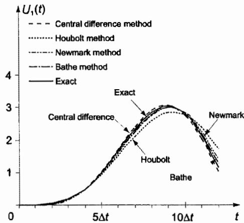
The results obtained are compared in Fig. E9.7 with the response predicted using the central difference, Houbolt, Newmark and Bathe methods in Examples 9.1 to 9.4, respectively. The discussion in Section 9.4 will show that the time step $\Delta t$ selected for the direct integrations is relatively large, and with this in mind it may be noted that the direct integration schemes predict a fair approximation to the exact response of the system.
Instead of evaluating the exact response as given in (d) we could use a numerical integration scheme to solve the equations in (a). Here we employ the Newmark method and obtain
line
| t | Central difference method | Houbolt method | Newmark method | Bathe method | Exact |
| ------- | ------------------------- | -------------- | -------------- | ------------ | ----- |
| 0 | 0.0 | 0.0 | 0.0 | 0.0 | 0.0 |
| 5Δt | ~1.5 | ~1.5 | ~1.5 | ~1.5 | ~1.5 |
| 10Δt | ~3.0 | ~3.0 | ~3.0 | ~3.0 | ~3.0 |
(a)
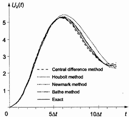
line
| t | Central difference method | Houbolt method | Newmark method | Bathe method | Exact |
|-------|---------------------------|----------------|----------------|--------------|-------|
| 0 | 0.0 | 0.0 | 0.0 | 0.0 | 0.0 |
| 5Δt | 5.5 | 5.6 | 5.4 | 5.3 | 5.5 |
| 10Δt | 2.5 | 2.6 | 2.4 | 2.3 | 2.5 |
(b)
Figure E9.7 Displacement response of system considered in Examples 9.1, 9.2, 9.3, 9.4, and 9.7
| Time | $\Delta t$ | $2\Delta t$ | $3\Delta t$ | $4\Delta t$ | $5\Delta t$ | $6\Delta t$ |
| $x_{1}(t)$ | 0.2178 | 0.8383 | 1.768 | 2.866 | 3.968 | 4.906 |
| $x_{2}(t)$ | -0.2915 | -1.062 | -2.036 | -2.867 | -3.257 | -3.067 |
| $7\Delta t$ | $8\Delta t$ | $9\Delta t$ | $10\Delta t$ | $11\Delta t$ | $12\Delta t$ |
| 5.540 | 5.773 | 5.571 | 4.964 | 4.043 | 2.948 |
| -2.365 | -1.402 | -0.5216 | -0.03776 | -0.1234 | -0.7480 |
The solution for $U_{1}(t)$ and $U_{2}(t)$ is now evaluated by substituting for $\mathbf{X}(t)$ in the relation given in (c). As expected, it is found that the displacement response thus predicted is the same as the response obtained when using the Newmark method in direct integration.
As discussed so far, the only difference between a mode superposition and a direct integration analysis is that prior to the time integration, a change of basis is carried out, namely, from the finite element coordinate basis to the basis of eigenvectors of the generalized eigenproblem $K\phi = \omega^{2}M\phi$ . Since mathematically the same space is spanned by the n eigenvectors as by the n nodal point finite element displacements, the same solution must be obtained in both analyses. The choice of whether to use direct integration or mode superposition will therefore be decided by considerations of effectiveness only. However, this choice can only be made once an important additional aspect of mode superposition has been presented. This aspect relates to the distribution and frequency content of the loading and renders the mode superposition solution of some structures much more effective than the use of direct integration.
Consider the decoupled equilibrium equations in (9.46). We note that if $r_{i}(t)=0$ , $i=1,\ldots,n$ , and either the initial displacements ${}^{0}U$ or the initial velocities ${}^{0}\dot{U}$ are a
multiple of $\phi_{j}$ , and only of $\phi_{j}$ , then only $x_{j}(t)$ is nonzero and the structure will vibrate only in this mode shape. In practice, such transient response will decrease in magnitude due to damping (see Section 9.3.3) and frequently the effect of the external loading is more important.
Therefore, consider next that ${}^{0}U = {}^{0}U = 0$ , and that the loading is of the form $\mathbf{R}(t) = \mathbf{M}\boldsymbol{\Phi}_{j}f(t)$ , where $f(t)$ is an arbitrary function of t. In such a case, since $\boldsymbol{\Phi}_{i}^{T}\mathbf{M}\boldsymbol{\Phi}_{j} = \delta_{ij}$ ( $\delta_{ij} = \text{Kronecker delta}$ ), we would have that only $x_{j}(t)$ is nonzero. These are rather stringent conditions, and in general analysis can hardly be expected to apply exactly to many of the n equations in (9.46) because the loading is in general arbitrary. However, in addition to the fact that the loading may be nearly orthogonal to $\phi_{i}$ , it is also the frequency content of the loading that determines whether the ith equation in (9.46) will contribute significantly to the response. Namely, the response $x_{i}(t)$ is relatively large if the excitation frequency contained in $r_{i}$ lies near $\omega_{i}$ .
To demonstrate these basic considerations we introduce the following example.
EXAMPLE 9.8: Consider a one degree of freedom system with the equilibrium equation
$$
\ddot {x} (t) + \omega^ {2} x (t) = R \sin \hat {\omega} t
$$
and initial conditions
$$
x \mid_ {t = 0} = 0, \quad \dot {x} \mid_ {t = 0} = 1 \tag {a}
$$
Use the Duhamel integral to calculate the displacement response.
We note that the system is subjected to a periodic force input and a nonzero initial velocity. Using the relation in (9.47), we obtain
$$
x (t) = \frac {R}{\omega} \int_ {0} ^ {t} \sin \hat {\omega} \tau \sin \omega (t - \tau) d \tau + \alpha \sin \omega t + \beta \cos \omega t
$$
Evaluating the integral, we obtain
$$
x (t) = \frac {R / \omega^ {2}}{1 - \hat {\omega} ^ {2} / \omega^ {2}} \sin \hat {\omega} t + \alpha \sin \omega t + \beta \cos \omega t \tag {b}
$$
We now need to use the initial conditions to evaluate $\alpha$ and $\beta$ . The solution at time t = 0 is
$$
x \mid_ {t = 0} = \beta
$$
$$
\dot {x} \mid_ {t = 0} = \frac {R \hat {\omega} / \omega^ {2}}{1 - \hat {\omega} ^ {2} / \omega^ {2}} + \alpha \omega
$$
Using the conditions in (a), we obtain
$$
\beta = 0; \quad \alpha = \frac {1}{\omega} - \frac {R \hat {\omega} / \omega^ {3}}{1 - \hat {\omega} ^ {2} / \omega^ {2}}
$$
Substituting for $\alpha$ and $\beta$ into (b), we thus have
$$
x (t) = \frac {R / \omega^ {2}}{1 - \hat {\omega} ^ {2} / \omega^ {2}} \sin \hat {\omega} t + \left(\frac {1}{\omega} - \frac {R \hat {\omega} / \omega^ {3}}{1 - \hat {\omega} ^ {2} / \omega^ {2}}\right) \sin \omega t
$$
which may also be written as
$$
x (t) = D x _ {\text { stat }} + x _ {\text { trans }}
$$
where $x_{stat}$ is the static response of the system,
$$
x _ {\text { stat }} = \frac {R}{\omega^ {2}} \sin \hat {\omega} t
$$
$x_{\mathrm{trans}}$ is the transient response,
$$
x _ {\text { trans }} = \left(\frac {1}{\omega} - \frac {R \hat {\omega} / \omega^ {3}}{1 - \hat {\omega} ^ {2} / \omega^ {2}}\right) \sin \omega t
$$
and $D$ is the dynamic load factor, indicating resonance when $\hat{\omega} = \omega$ ,
$$
D = \frac {1}{1 - \hat {\omega} ^ {2} / \omega^ {2}}
$$
The analysis of the response of the single degree of freedom system considered in this example showed that the complete response is the sum of two contributions:
1. A dynamic response obtained by multiplying the static response by a dynamic load factor (this is the particular solution of the governing differential equation), and
2. An additional dynamic response which we called the transient response.
These observations pertain also to an actual practical analysis of a multiple degree of freedom system because, first, the complete response is obtained as a superposition of the response measured in each modal degree of freedom, and second, the actual loading can be represented in a Fourier decomposition as a superposition of harmonic sine and cosine contributions. Therefore, the above two observations apply to each modal response corresponding to each Fourier component of the loading.
An important difference between an actual practical response analysis and the solution in Example 9.8 is, however, that in practice the effect of damping must be included as discussed in Section 9.3.3. The presence of damping reduces the dynamic load factor (which then cannot be infinite) and damps out the transient response.
Figure 9.3 shows the dynamic load factor as a function of $\hat{\omega}/\omega$ (and the damping ratio $\xi$ discussed in Section 9.3.3). The information in Fig. 9.3 is obtained by solving (9.54) as in Example 9.8. If we apply the information given in this figure to the analysis of an actual practical system, we recognize that the response in the modes with $\hat{\omega}/\omega$ large is negligible (the loads vary so rapidly that the system does not move), and that the static response is measured when $\hat{\omega}/\omega$ is close to zero (the loads vary so slowly that the system simply follows the loads statically). Therefore, in the analysis of a multiple degree of freedom system, the response in the high frequencies of the system (that are much larger than the highest frequencies contained in the loads) is simply a static response.
The essence of a mode superposition solution of a dynamic response is that frequently only a small fraction of the total number of decoupled equations needs to be considered in order to obtain a good approximate solution to the exact solution of (9.1). Most frequently, only the first $p$ equilibrium equations in (9.46) need to be used; i.e., we need to include in the analysis the equations (9.46) only for $i = 1, 2, \ldots, p$ , where $p \ll n$ , in order to obtain a good approximate solution. This means that we need to solve only for the lowest $p$ eigenvalues and corresponding eigenvectors of the problem in (9.36) and we only sum in