# THE STIFFNESS METHOD AND THE # PLANE TRUSS Matrix procedures used in the analysis of framed structures and other finite element structures are described. The plane truss is used as the principal vehicle for the discussion. # 2.1 INTRODUCTION Certain matrix procedures of structural mechanics are described in this chapter. These methods are also used in finite element analysis of many other physical problems. These procedures include assembly of elements to form a structure, imposition of boundary or support conditions, solution of simultaneous equations to obtain nodal quantities, and processing of elements to obtain quantities such as stresses or flows. The plane truss is a very simple structure that serves to explain these concepts and procedures. The truss can be called a “discrete element” structure. Its elements are the individual bars, already present as separate pieces. Thus we bypass the important finite element processes of dividing a continuum into appropriate elements and idealizing the behavior of each element. In the present chapter we are primarily concerned with manipulation procedures that apply to a previously discretized structure. Each bar of a truss is assumed to be uniform, linearly elastic, pin-connected to nodes at its ends, and axially loaded. Displacements shown in sketches are greatly exaggerated. Actual displacements are assumed to be small, so that if $\theta$ is the angle of rotation under load of any bar, then $\sin \theta \approx \theta$ and $\cos \theta \approx 1$ . We consider only statically loaded structures. Within these restrictions, the analysis is exact, not approximate. Degrees of Freedom (d.o.f.). A structure has n d.o.f. if n independent quantities are needed to uniquely define the deformed configuration of the structure. The structure stiffness matrix will have n rows and n columns. In a plane truss, n is equal to two times the number of nodes allowed to displace. The individual d.o.f. are the x- and y-direction displacement components of each structure node. In nonstructural problems, d.o.f. are analogously defined: they are the independent quantities needed to define a field, such as the temperature field in a heat conduction problem. In heat conduction analysis, there is a single d.o.f. per node—namely, the nodal temperature. # 2.2 STRUCTURE STIFFNESS EQUATIONS We begin by generating the structure stiffness matrix [K] of a plane truss by a direct attack on the structure as a whole. The result will be used to illustrate certain concepts. Later we will show how [K] can be built by assembly of element matrices, which is the process actually used in computer programs. 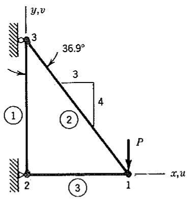Consider, for example, the three-bar truss of Fig. 2.2-1. Nodes and elements (bars) are numbered arbitrarily. For element i, where i = 1, 2, 3 in this example, let $A_{i} = \text{cross-sectional area}$ , $E_{i} = \text{elastic modulus}$ , and $L_{i} = \text{length}$ . From elementary mechanics of materials, axial force $F_{i}$ and change in length $e_{i}$ have the relation $$ \sqrt {e _ {i}} = \frac {F _ {i} L _ {i}}{A _ {i} E _ {i}} \tag {2.2-1} $$ Stiffness is defined as the ratio of force to displacement and is by custom given the symbol k. 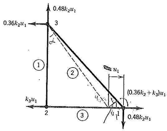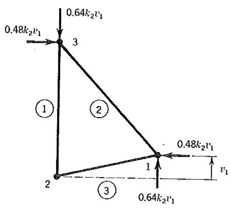Thus, the axial stiffness of any uniform bar of a truss is $$ \sqrt {k _ {i}} = \frac {F _ {i}}{e _ {i}} = \frac {A _ {i} E _ {i}}{L _ {i}} \tag {2.2-2} $$ Supports at nodes 2 and 3 in Fig. 2.2-1 are temporarily removed, so that nonzero values can be assigned to all nodal displacements. Now let a node be displaced a small amount, first in the x direction and then in the y direction, while all other nodes are held at zero displacement. Thus there are six possible deformation states for a three-node plane truss. In each of these six states we calculate forces that must be applied to the nodes to maintain the deformation state. These forces, acting on the truss cut free of its supports, place the truss in static equilibrium. The first two free-body diagrams are shown in Fig. 2.2-2. As an example of the force computation, consider the forces in Fig. 2.2-2a. Because displacement $u_{1}$ is small, its component along bar 2, which is the change in length of bar 2, is $e_{2} = 0.6u_{1}$ . This deformation produces the axial force $F_{2} = k_{2}e_{2}$ , whose horizontal and vertical components have the respective magnitudes $0.6F_{2} = 0.36k_{2}u_{1}$ and $0.8F_{2} = 0.48k_{2}u_{1}$ . Bar 3 has elongation $e_{3} = u_{1}$ and contributes forces $F_{3} = k_{3}e_{3} = k_{3}u_{1}$ . 

text_image

y,v 3 36.9° 3 4 ① ② P 2 ③ 1 x,u

Figure 2.2-1. A three-bar plane truss. D.o.f. $u_{2}$ , $v_{2}$ , and $u_{3}$ are restrained. D.o.f. $u_{1}$ , $v_{1}$ , and $v_{3}$ are active (allowed to displace). Externally applied loading consists of force P. 

text_image

0.48k₂u₁ 0.36k₂u₁ 3 ① ② u₁ (0.36k₂ + k₃)u₁ k₃u₁ 2 ③ u₁ 0.48k₂u₁

(a) 

text_image

0.64k₂v₁ 0.48k₂v₁ 3 ① ② 0.48k₂v₁ 1 2 ③ 0.64k₂v₁ v₁

(b) Figure 2.2-2. Nodal loads consistent with the respective displacement states $\{\mathbf{D}\} = [u_1 0 0 0 0 0]^T$ and $\{\mathbf{D}\} = [0 v_1 0 0 0 0]^T$ . Let $\{\mathbf{Q}_1\}$ represent the vector of forces in Fig. 2.2-2a associated with unit displacement, $u_1 = 1$ . Thus forces that appear in Fig. 2.2-2a are $\{\mathbf{Q}_1\} u_1$ : $$ \left\{\mathbf {Q} _ {1} \right\} u _ {1} = \left\lfloor k _ {3} + 0. 3 6 k _ {2} - 0. 4 8 k _ {2} - k _ {3} 0 - 0. 3 6 k _ {2} 0. 4 8 k _ {2} \right] ^ {T} u _ {1} \tag {2.2-3} $$ Similarly, forces that appear in Fig. 2.2-2b are $\{Q_{2}\}v_{1}$ , where $\{Q_{2}\}$ is the force vector associated with the unit displacement $v_{1}=1$ : $$ \{\mathbf {Q} _ {2} \} v _ {1} = \left[ - 0. 4 8 k _ {2} \quad 0. 6 4 k _ {2} \quad 0 \quad 0 \quad 0. 4 8 k _ {2} \quad - 0. 6 4 k _ {2} \right] ^ {T} v _ {1} \tag {2.2-4} $$ Let $\{\mathbf{Q}_3\}, \{\mathbf{Q}_4\}, \{\mathbf{Q}_5\}$ , and $\{\mathbf{Q}_6\}$ represent the equilibrium nodal force vectors associated with the remaining four unit displacement states $u_2 = 1$ , $v_2 = 1$ , $u_3 = 1$ , and $v_3 = 1$ . Then, if all six nodal d.o.f. may be nonzero simultaneously, the associated nodal loads are obtained by adding the six separate cases, $$ \left[ \begin{array}{l l l l l l} \mathbf {Q} _ {1} & \mathbf {Q} _ {2} & \mathbf {Q} _ {3} & \mathbf {Q} _ {4} & \mathbf {Q} _ {5} & \mathbf {Q} _ {6} \end{array} \right] \left\{ \begin{array}{l} u _ {1} \\ v _ {1} \\ u _ {2} \\ v _ {2} \\ u _ {3} \\ v _ {3} \end{array} \right\} = \left\{ \begin{array}{l} p _ {1} \\ q _ {1} \\ p _ {2} \\ q _ {2} \\ p _ {3} \\ q _ {3} \end{array} \right\} \tag {2.2-5} $$ where forces applied to node i are called $p_{i}$ and $q_{i}$ , positive in +x and +y directions, respectively. Written out, Eq. 2.2-5 is $$ \left[ \begin{array}{c c c c c c} k _ {3} + 0. 3 6 k _ {2} & - 0. 4 8 k _ {2} & - k _ {3} & 0 & - 0. 3 6 k _ {2} & 0. 4 8 k _ {2} \\ - 0. 4 8 k _ {2} & 0. 6 4 k _ {2} & 0 & 0 & 0. 4 8 k _ {2} & - 0. 6 4 k _ {2} \\ - k _ {3} & 0 & k _ {3} & 0 & 0 & 0 \\ 0 & 0 & 0 & k _ {1} & 0 & - k _ {1} \\ - 0. 3 6 k _ {2} & 0. 4 8 k _ {2} & 0 & 0 & 0. 3 6 k _ {2} & - 0. 4 8 k _ {2} \\ 0. 4 8 k _ {2} & - 0. 6 4 k _ {2} & 0 & - k _ {1} & - 0. 4 8 k _ {2} & k _ {1} + 0. 6 4 k _ {2} \end{array} \right] \left\{ \begin{array}{l} u _ {1} \\ \widehat {v _ {1}} \\ u _ {2} \\ v _ {2} \\ u _ {3} \\ v _ {3} \end{array} \right\} = \left\{ \begin{array}{l} p _ {1} \\ q _ {1} \\ p _ {2} \\ q _ {2} \\ p _ {3} \\ q _ {3} \end{array} \right\} \tag {2.2-6} $$ In our standard abbreviation, these structure stiffness equations are $$ [ \mathbf {K} ] \{\mathbf {D} \} = \{\mathbf {R} \} \tag {2.2-7} $$ where [K] is the structure stiffness matrix. As shown by the development, Eqs. 2.2-7 are equilibrium equations. The physical meaning of [K], as well as a procedure for formulating [K], are contained in the following statement. The jth column of [K] is the vector of loads that must be applied to nodal d.o.f. in order to maintain the deformation state associated with unit value of d.o.f. j while all other nodal d.o.f. are zero. For a frame, “loads” include displacements and rotations. By this procedure—activating one d.o.f. at a time—we can generate the stiffness matrix of any truss or frame, regardless of the number of bars or the degree of static indeterminacy. The stiffness matrix is square; that is, there are as many equations as there are d.o.f. # 2.3 PROPERTIES OF [K]. SOLUTION FOR UNKNOWNS Properties of [K]. Each diagonal stiffness coefficient $K_{ii}$ in Eq. 2.2-6 is positive. This is physically reasonable, as it means that a force $R_{i}$ directed toward (say) the right will not produce a displacement directed toward the left (here it helps to imagine that all d.o.f. in {D} except $D_{i}$ are constrained to be zero). In general, for any structure, no diagonal coefficient $K_{ii}$ is negative or zero unless the structure is unstable. [ K ] is symmetric. This is true of any structure that displays a linear relationship between applied loads and the resulting displacements. The symmetry of [K] may be proved by use of the procedure suggested in Problem 2.7. If the structure is not attached to supports, its [K] does not resist rigid-body motion of the structure. An infinite number of vectors $\{\mathbf{D}\}$ that represent rigid-body motion can be written. For the plane truss of Fig. 2.2-1, with all supports removed, four of them are $$ \{\mathbf {D} \} _ {1} = \left[ \begin{array}{l l l l l l} \delta & 0 & \delta & 0 & \delta & 0 \end{array} \right] ^ {T} \quad \{\mathbf {D} \} _ {2} = \left[ \begin{array}{l l l l l l} 0 & \delta & 0 & \delta & 0 & \delta \end{array} \right] ^ {T} \tag {2.3-1} $$ $$ \{\mathbf {D} \} _ {3} = \left[ \begin{array}{c c c c c c} \delta & \delta & \delta & \delta & \delta & \delta \end{array} \right] ^ {T} \quad \{\mathbf {D} \} _ {4} = \left[ \begin{array}{c c c c c c} 4 \theta & 3 \theta & 4 \theta & 0 & 0 & 0 \end{array} \right] ^ {T} $$ where $\delta$ is a small displacement and $\theta$ is a small angle of rotation. Respectively, the foregoing vectors represent translation along the $x$ axis, translation along the $y$ axis, translation along the line $x = y$ , and rotation about node 3. For any plane structure only three of the infinitely many rigid-body $\{\mathbf{D}\}_{i}$ are linearly independent. The choice of three is not unique. For example, from Eqs. 2.3-1 we could choose $\{\mathbf{D}\}_{4}$ and any two of $\{\mathbf{D}\}_{1}, \{\mathbf{D}\}_{2}$ , and $\{\mathbf{D}\}_{3}$ . The first three $\{\mathbf{D}\}_{i}$ in Eqs. 2.3-1 are linearly dependent because $\{\mathbf{D}\}_{3} = \{\mathbf{D}\}_{i} + \{\mathbf{D}\}_{2}$ . A rigid-body motion does not deform a structure. Therefore, $[\mathbf{K}]\{\mathbf{D}\}_{i} = \{\mathbf{0}\}$ for any rigid-body motion $\{\mathbf{D}\}_{i}$ . With reference to our three-bar truss example, and for $\delta = 1$ in Eqs. 2.3-1, the equations $[\mathbf{K}]\{\mathbf{D}\}_{3} = \{\mathbf{0}\}$ state that coefficients in each row of $[\mathbf{K}]$ sum to zero. Note, however, that row sums of $[\mathbf{K}]$ will not vanish for any and all structures, since setting each entry in $\{\mathbf{D}\}$ to unity does not in general constitute rigid-body motion. Cases in point include structures that contain beam or plate elements, for which rotational d.o.f. are present. To summarize: for an unsupported structure, (a) $[K]\{D\} = \{0\}$ when $\{D\}$ represents rigid-body motion, and (b) each column of $[K]$ represents a set of nodal forces and/or moments in static equilibrium. Solution for Unknowns. The stiffness matrix of Eq. 2.2-6 is singular. Its order is 6 but its rank is 3. [K] cannot be inverted, nor can a unique {D} be obtained by solving equations. The physical reason for this is that rigid-body motion is still possible. Without supports, the structure will float away if the slightest external load is applied. Before continuing with the truss example we state a more general argument about solution for unknowns, as follows. One must remove the singularity of [K] in order to solve for the unknown d.o.f. in {D}. We now show a formal procedure by which this may be done. Let $\{\mathbf{D}_c\}$ and $\{\mathbf{R}_c\}$ be known d.o.f. and known loads, and $\{\mathbf{D}_x\}$ and $\{\mathbf{R}_x\}$ be as yet unknown d.o.f. and loads. By partitioning, accompanied by such rearrangement of matrix coefficients as may be necessary, the structural equations [K]{D} = {R} can be written in the form $$ \left[ \begin{array}{l l} \mathbf {K} _ {1 1} & \mathbf {K} _ {1 2} \\ \mathbf {K} _ {2 1} & \mathbf {K} _ {2 2} \end{array} \right] \left\{ \begin{array}{l} \mathbf {D} _ {x} \\ \mathbf {D} _ {c} \end{array} \right\} = \left\{ \begin{array}{l} \mathbf {R} _ {c} \\ \mathbf {R} _ {x} \end{array} \right\} \tag {2.3-2} $$ or, in a more expanded form, $$ [ \mathbf {K} _ {1 1} ] \{\mathbf {D} _ {x} \} + [ \mathbf {K} _ {1 2} ] \{\mathbf {D} _ {c} \} = \{\mathbf {R} _ {c} \} \tag {2.3-3} $$ $$ [ \mathbf {K} _ {2 1} ] \{\mathbf {D} _ {x} \} + [ \mathbf {K} _ {2 2} ] \{\mathbf {D} _ {c} \} = \{\mathbf {R} _ {x} \} \tag {2.3-4} $$ (Note that at this stage we know either a d.o.f. or its corresponding load, but not both.) $[K_{11}]$ is nonsingular if the prescribed d.o.f. $\{D_{c}\}$ are sufficient in arrangement and number to prevent rigid-body motion. Therefore, the unknown d.o.f. $\{D_{x}\}$ can be found from Eq. 2.3-3: $$ \{\mathbf {D} _ {x} \} = [ \mathbf {K} _ {1 1} ] ^ {- 1} \left(\{\mathbf {R} _ {c} \} - [ \mathbf {K} _ {1 2} ] \{\mathbf {D} _ {c} \}\right) \tag {2.3-5} $$ Finally, unknown loads $\{R_{x}\}$ can be found from Eq. 2.3-4 after substitution of d.o.f. $\{D_{x}\}$ , which are now known. In structural mechanics, $\{R_{x}\}$ usually represents support reactions. In practice, the foregoing rearrangement of coefficients, partitioning, and matrix inversion are avoided by use of other operations that implicitly accomplish the same ends. These operations are discussed in Section 2.10. We now apply the foregoing solution procedure to the truss of Fig. 2.2-1. Support conditions $\{\mathbf{D}_c\}$ are $$ u _ {2} = v _ {2} = u _ {3} = 0 \quad \checkmark \tag {2.3-6} $$ which means that $\{\mathbf{D}_c\} = \{\mathbf{0}\}$ . Known loads $\{\mathbf{R}_c\}$ , which correspond to as yet unknown d.o.f., are $$ p _ {1} = 0 \quad q _ {1} = - P \quad q _ {3} = 0 \tag {2.3-7} $$ Equation 2.3-3 becomes $[\mathbf{K}_{11}]\{\mathbf{D}_x\} = \{\mathbf{R}_c\}$ , or $$ \left[ \begin{array}{c c c} k _ {3} + 0. 3 6 k _ {2} & - 0. 4 8 k _ {2} & 0. 4 8 k _ {2} \\ - 0. 4 8 k _ {2} & 0. 6 4 k _ {2} & - 0. 6 4 k _ {2} \\ 0. 4 8 k _ {2} & - 0. 6 4 k _ {2} & k _ {1} + 0. 6 4 k _ {2} \end{array} \right] \left\{ \begin{array}{l} u _ {1} \\ v _ {1} \\ v _ {3} \end{array} \right\} = \left\{ \begin{array}{c} 0 \\ - P \\ 0 \end{array} \right\} \tag {2.3-8} $$ Since $[K_{11}]$ is nonsingular, Eq. 2.3-8 has a unique solution and can be solved for $u_{1}$ , $v_{1}$ , and $v_{3}$ . Then, since $\{D_{c}\} = \{0\}$ , Eq. 2.3-4 becomes $\{R_{x}\} = [K_{21}]\{D_{x}\}$ , or $$ \left\{ \begin{array}{l} p _ {2} \\ q _ {2} \\ p _ {3} \end{array} \right\} = \left[ \begin{array}{c c c} - k _ {3} & 0 & 0 \\ 0 & 0 & - k _ {1} \\ - 0. 3 6 k _ {2} & 0. 4 8 k _ {2} & - 0. 4 8 k _ {2} \end{array} \right] \left\{ \begin{array}{l} u _ {1} \\ v _ {1} \\ v _ {3} \end{array} \right\} \tag {2.3-9} $$ which can be solved for the support reactions $p_2, q_2$ , and $p_3$ by substituting the known values of $u_1, v_1$ , and $v_3$ . The case $\{\mathbf{D}_c\} = \{\mathbf{0}\}$ , which says that all prescribed d.o.f. are zero, is common. When $\{\mathbf{D}_c\} = \{\mathbf{0}\}$ one can obtain $[\mathbf{K}_{11}]$ from $[\mathbf{K}]$ by discarding each row $i$ and column $i$ for which $D_i = 0$ . In the present example problem, we obtain Eq. 2.3-8 by discarding rows and columns 3, 4, and 5 from Eq. 2.2-6. Note also that $[K_{11}]$ can be obtained by applying the procedure described in Section 2.2, using only active d.o.f. and calculating loads associated with these d.o.f. Thus, for the truss of Fig. 2.2-1, one obtains the first column of $[K_{11}]$ by setting $u_{1}=1$ and $u_{2}=v_{2}=u_{3}=0$ , then computing the nodal loads $p_{1}, q_{1}$ , and $q_{3}$ . $$ \begin{array}{l} p u ^ {k} \\ 3 8 3 \end{array} $$ # 2.4 ELEMENT STIFFNESS EQUATIONS In Section 2.2, [K] is generated directly by considering the structure as a whole. This approach clarifies the physical meaning of [K] but does not lend itself to computer implementation. In practice, [K] is built by summation of coefficients from element stiffness matrices [k]. The summation process is easily computerized. In the present section we formulate the necessary element [k] matrix for a uniform plane truss member. 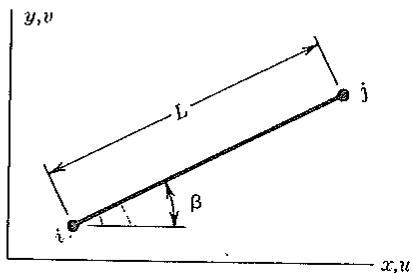Let the element of Fig. 2.4-1 have constant cross-sectional area $A$ and elastic modulus $E$ . Everything needed to generate [k] can be found from $A, E$ , and the four nodal coordinates $x_{i}, x_{j}, y_{i}$ , and $y_{j}$ . First, we compute $$ L = [ (x _ {j} - x _ {i}) ^ {2} + (y _ {j} - y _ {i}) ^ {2} ] ^ {1 / 2} \tag {2.4-1a} $$ $$ s = \sin \beta = \frac {y _ {j} - y _ {i}}{L}. 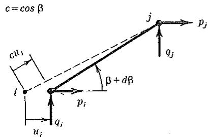\tag {2.4-1b} $$ $$ c = \cos \beta = \frac {x _ {j} - x _ {i}}{L} \tag {2.4-1c} $$ Next, as in Section 2.2, we generate columns of [k] by activating each d.o.f. in turn while keeping the others zero. The first of these four cases is shown in Fig. 2.4-2. Axial shortening $cu_{i}$ produces an axial compressive force $F = (AE/L)cu_{i}$ , 

text_image

y,v L j i β x,u

Figure 2.4-1. A uniform truss element, arbitrarily oriented in the xy plane. 

text_image

c = cos β j p_j q_j β + dβ p_i u_i q_i i c u_i

Figure 2.4-2. The truss element after nodal displacements $u_{i} > 0$ , $v_{i} = u_{j} = v_{j} = 0$ have been imposed. whose $x$ and $y$ components are $p_i = -p_j = Fc$ and $q_i = -q_j = Fs$ . These components provide static equilibrium. Thus $$ \frac {A E}{L} \left\{ \begin{array}{l} c ^ {2} \\ c s \\ - c ^ {2} \\ - c s \end{array} \right\} u _ {i} = \left\{ \begin{array}{l} p _ {i} \\ q _ {i} \\ p _ {j} \\ q _ {j} \end{array} \right\} \tag {2.4-2} $$ Similar results are given by the remaining displacements, $v_{i}$ , $u_{j}$ , and $v_{j}$ , when each acts alone. If all four d.o.f. may be nonzero simultaneously, we superpose results, just as in Eq. 2.2-5, and obtain $$ \frac {A E}{L} \left[ \begin{array}{c c c c} c ^ {2} & c s & - c ^ {2} & - c s \\ c s & s ^ {2} & - c s & - s ^ {2} \\ - c ^ {2} & - c s & c ^ {2} & c s \\ - c s & - s ^ {2} & c s & s ^ {2} \end{array} \right] \left\{ \begin{array}{l} u _ {i} \\ v _ {i} \\ u _ {j} \\ v _ {j} \end{array} \right\} = \left\{ \begin{array}{l} p _ {i} \\ q _ {i} \\ p _ {j} \\ q _ {j} \end{array} \right\} \tag {2.4-3} $$ where $c = \cos \beta$ and $s = \sin \beta$ . The square matrix, including the factor $AE / L$ , is the element stiffness matrix [k]. We abbreviate Eq. 2.4-3 as $$ [ \mathbf {k} ] \{\mathbf {d} \} = \{\widetilde {\mathbf {r}} \} \tag {2.4-4} $$ The jth column of [k] is the vector of loads that must be applied to element nodes to maintain the deformation state when $d_{j} = 1$ and all other element nodal d.o.f. are zero. Subsequently it will be desirable to distinguish between loads applied by the element and loads applied to the element. Loads $\{\bar{\mathbf{r}}\} = [\mathbf{k}]\{\mathbf{d}\}$ are applied to the element in order to sustain nodal d.o.f. $\{\mathbf{d}\}$ . Why are rotational d.o.f. not present in $\{d\}$ ? Such d.o.f. would be present if bending stiffness of the bar were taken into account. Then the structure would be a beam or a plane frame. By definition, truss bars do not resist bending. In a truss, rotational d.o.f. are not introduced because there is no resistance to them. Their presence would make $[K]$ a singular matrix. Special Cases. If $\beta = 0$ , as for bar 3 in Fig. 2.2-1, [k] remains 4 by 4 but contains only four nonzero coefficients, $k_{11} = k_{33} = -k_{13} = -k_{31} = AE / L$ . Therefore, displacements $v_{i}$ and $v_{j}$ produce no nodal loads $\{\overline{\mathbf{r}}\}$ . This is correct: in accordance with our assumptions, small lateral displacements $v_{i}$ and $v_{j}$ do not strain the bar and therefore generate no force. Similar remarks apply if $\beta = \pi / 2$ , $\pi$ , and so on. That some diagonal coefficients in [k] are null does not necessarily mean that any diagonal coefficient in the assembled [K] will be null. Imagine that $\beta = 0$ and that $v_{i}$ and $v_{j}$ are suppressed by striking out rows and columns 2 and 4 from Eq. 2.4-3. What remains is $$ \frac {A E}{L} \left[ \begin{array}{c c} 1 & - 1 \\ - 1 & 1 \end{array} \right] \left\{ \begin{array}{l} u _ {i} \\ u _ {j} \end{array} \right\} = \left\{ \begin{array}{l} p _ {i} \\ p _ {j} \end{array} \right\} \tag {2.4-5} $$ This is the stiffness equation of a bar allowed only the axial d.o.f. $u_{i}$ and $u_{j}$ . It was previously derived (Eq. 1.2-3). The orientation of the bar in space does not matter if $u_{i}, u_{j}, p_{i}$ , and $p_{j}$ remain axially directed. In Section 7.5 we will see that Eq. 2.4-3 can be obtained from Eq. 2.4-5 by a simple coordinate transformation procedure. The 2 by 2 stiffness matrix in Eq. 2.4-5 is used in various examples throughout this book. $$ \begin{array}{l} p _ {0} ^ {\prime} C \\ 3 8 3 \end{array} $$ # 2.5 ASSEMBLY OF ELEMENTS. PLANE TRUSS EXAMPLE The process of assembling elements to form a structure can be symbolized as $[\mathbf{K}] = \Sigma[\mathbf{k}]$ . In this section we consider arguments that apply to the three-bar truss of Fig. 2.2-1. In subsequent sections we present more general arguments and provide computer algorithms. Fortunately, the concepts and procedures of assembly depend very little on whether the structure is a truss, a frame, or a discretized continuum. Physically, construction of the truss of Fig. 2.2-1 can be visualized as follows. Structure nodes are positioned in space and are assigned labels, such as 1, 2, and 3 in Fig. 2.2-1. Bars are at first unassembled, but each bar is tagged with a node label at each end to show where it is to be placed. One by one, the bars are attached to the appropriate structure nodes. The structure gains stiffness as each bar is added. Symbolically, the foregoing process is that of starting with a null structure stiffness matrix [K], then adding to it the [k] of each element. When the last element has been added, the structure is complete and [K] is complete. The summation $[K] = \Sigma [k]$ can be performed if each $[k]$ is made to operate on $\{D\}$ , the vector of structure d.o.f. If the structure has n d.o.f., this means that each $[k]$ must be expanded to become an n by n matrix. Such expansion to “structure size” is a helpful conceptual device. Computationally it would be cumbersome. In Section 2.7 we will show how to perform the summation without expansion. To begin, we write [k] for each bar in Fig. 2.2-1 as a 4 by 4 matrix. Element node labels $i$ and $j$ can be interchanged: in other words, adding $\pi$ to angle $\beta$ does not change Eq. 2.4-3. To this extent, node labels on the bars are arbitrary. Let $k_{1}, k_{2}$ , and $k_{3}$ represent the $AE/L$ factors of the respective bars, and apply Eq. 2.4-3. Bar 1: Let $i = 2$ and $j = 3$ . Hence $\beta = 90^{\circ}$ , $c = 0$ , and $s = 1$ . $$ [ \mathbf {k} ] _ {1} \{\mathbf {d} \} _ {1} = k _ {1} \left[ \begin{array}{c c c c} 0 & 0 & 0 & 0 \\ 0 & 1 & 0 & - 1 \\ 0 & 0 & 0 & 0 \\ 0 & - 1 & 0 & 1 \end{array} \right] \left\{ \begin{array}{l} u _ {2} \\ v _ {2} \\ u _ {3} \\ v _ {3} \end{array} \right\} \tag {2.5-1} $$ Bar 2: Let $i = 1$ and $j = 3$ . Hence $\beta = 126.9^{\circ}$ , $c = -0.6$ , and $s = 0.8$ . $$ [ \mathbf {k} ] _ {2} \{\mathbf {d} \} _ {2} = k _ {2} \left[ \begin{array}{c c c c} 0. 3 6 & - 0. 4 8 & 0. 3 6 & 0. 4 8 \\ - 0. 4 8 & 0. 6 4 & 0. 4 8 & - 0. 6 4 \\ - 0. 3 6 & 0. 4 8 & 0. 3 6 & - 0. 4 8 \\ 0. 4 8 & - 0. 6 4 & 0. 4 8 & 0. 6 4 \end{array} \right] \left\{ \begin{array}{l} u _ {1} \\ v _ {1} \\ u _ {3} \\ v _ {3} \end{array} \right\} \tag {2.5-2} $$ Bar 3: Let $i = 1$ and $j = 2$ . Hence $\beta = 180^{\circ}$ , $c = -1$ , and $s = 0$ . $$ [ \mathbf {k} ] _ {3} \{\mathbf {d} \} _ {3} = k _ {3} \left[ \begin{array}{c c c c} 1 & 0 & - 1 & 0 \\ 0 & 0 & 0 & 0 \\ - 1 & 0 & 1 & 0 \\ 0 & 0 & 0 & 0 \end{array} \right] \left\{ \begin{array}{l} u _ {1} \\ v _ {1} \\ u _ {2} \\ v _ {2} \end{array} \right\} \tag {2.5-3} $$ Each of the foregoing three [k] matrices must be expanded from 4 by 4 to 6 by 6. This is done by adding two rows of zeros and two columns of zeros—at the start in Eq. 2.5-1, in the middle in Eq. 2.5-2, and at the end in Eq. 2.5-3. Thus each element displacement vector becomes identical to the structure displacement vector {D}: $$ \left| \begin{array}{c c} \left. \begin{array}{c c c c c c} \mathbf {g} _ {1} & \varepsilon^ {\prime} \rho_ {m a x} \dot {\varepsilon} ^ {d} & \dot {\varepsilon} \varepsilon^ {l} & \rho_ {m a x} ^ {2} & \mathcal {L} _ {f} ^ {j} & \nu_ {m a x} ^ {i} \\ \hline \{\mathbf {d} \} _ {1} = \{\mathbf {d} \} _ {2} = \{\mathbf {d} \} _ {3} = \{\mathbf {D} \} = \left\lfloor u _ {1} v _ {1} u _ {2} v _ {2} u _ {3} v _ {3} \right\rfloor^ {T} & \end{array} \right. & \sqrt {\frac {1}{2} \frac {1}{2} \frac {1}{2}} \\ \hline \end{array} \right. $$ Equation 2.5-4 enforces compatibility; that is, it makes end points of the pin-connected bars coincident under any displacement $\{D\}$ . The addition of rows and columns of zeros can be physically justified as follows. Consider, for example, the expanded [k] of element 2, in which rows 3 and 4 and columns 3 and 4 contain only zeros. Element 2 and node 2 are not connected. Therefore, no displacement of node 2 can strain element 2. Thus displacements $u_{2}$ and $v_{2}$ are associated with zero force, which accounts for the two columns of zeros. In addition, none of the six d.o.f. can produce forces at node 2 because there is no connecting material to resist strain or transmit load. This accounts for the two rows of zeros. The reader can easily check that the expanded [k]'s from Eqs. 2.5-1, 2.5-2, and 2.5-3 do indeed add up to the structure [K] in Eq. 2.2-6. When one regards a column of [K] as a set of resisting forces, with each contributory force coming from elements connected to a common node, it becomes clear that one obtains [K] by adding element stiffness matrices. Stiffness Coefficients That Remain Zero. When is $K_{ij} = 0$ in the assembled structure? A column of [K] represents nodal loads associated with activation of one and only one d.o.f. Activation of a d.o.f. creates nodal loads in only the element or elements that contain the d.o.f. in question. Other elements are not strained and produce no nodal loads. Therefore, in a column $j$ of [K], coefficient $K_{ij}$ is zero unless structure d.o.f. i and j are both present in at least one element. ( $K_{ij}$ may be zero even if d.o.f. i and j are shared by an element. For example, in Eq. 2.2-6, $K_{41} = K_{14} = 0$ because/bar 3 of the truss happens to be horizontal.) # 2.6 ASSEMBLY REGARDED AS SATISFYING EQUILIBRIUM $$ \begin{array}{r l} {\mathrm {d} \theta} & {= \mathrm {d} \theta^ {\prime} / \mathrm {d} \theta^ {\prime} / \mathrm {d} \theta^ {\prime} / \mathrm {d} \theta^ {\prime} / \mathrm {d} \theta^ {\prime}} \\ {\mathrm {d} \theta} & {= \mathrm {d} \theta^ {\prime} / \mathrm {d} \theta^ {\prime} / \mathrm {d} \theta^ {\prime} / \mathrm {d} \theta^ {\prime} / \mathrm {d} \theta^ {\prime}} \end{array} $$ In stress analysis, assembly of elements can be regarded as a process of writing equations stating that each node of the structure is in static equilibrium under all loads applied to it. Nodal loads come from elements because of self-weight, temperature change, and lack of fit, from deformations associated with nodal displacements, and from external sources. The equilibrium argument is now explained with particular reference to the plane truss. 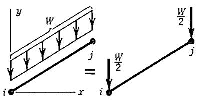Loads applied to nodes because of gravity in the negative y direction are shown in Fig. 2.6-1a. Written formally for a four d.o.f. 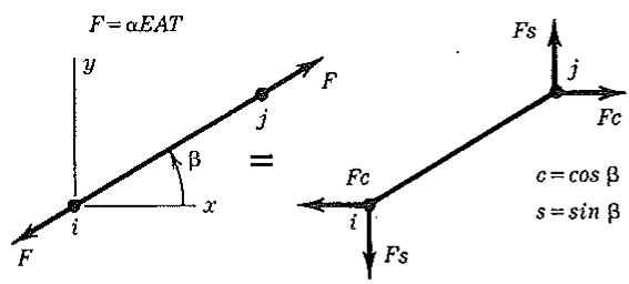element, these loads are $$ \{\mathbf {r} _ {w} \} = \frac {W}{2} \left[ \begin{array}{l l l l} 0 & - 1 & 0 & - 1 \end{array} \right] ^ {T} \tag {2.6-1} $$ where the total element weight W is equally apportioned to the two nodes. (We will assume that bending of an individual bar under its own weight can be neglected.) If a fully restrained bar is initially stress-free and then is uniformly heated T degrees, it sustains an axial compressive force $F = \alpha EAT$ , where $\alpha$ is the coefficient of thermal expansion (Fig. 2.6-1b). The resulting nodal load vector is $$ \{\mathbf {r} _ {T} \} = \alpha E A T \left[ - c - s c s \right] ^ {T} \tag {2.6-2} $$ where $c = \cos \beta$ and $s = \sin \beta$ . The same forces $\{r_{T}\}$ would arise from the force-fitting of a bar that is initially $\alpha LT$ units too long. We will use $\{r_{e}\}$ to symbolize element loads. For the loads mentioned here, $$ \{\mathbf {r} _ {e} \} = \{\mathbf {r} _ {W} \} + \{\mathbf {r} _ {T} \} \tag {2.6-3} $$ Loads $\{\tilde{r}\} = [k]\{d\}$ are loads applied to an element to sustain its deformation state $\{d\}$ . Therefore, equal and opposite loads $\{r\} = -\{\tilde{r}\}$ are applied by the element 

text_image

y W j = W/2 j i x i

(a) 

text_image

F = αEAT y β x i F F j F Fc Fc i Fs Fs j Fc c = cos β s = sin β

(b) Figure 2.6-1. (a) Allocation of the weight W of a truss bar to its nodes. (b) Nodal loads associated with uniform heating of T degrees above the unstressed temperature.