$$
\frac {\partial \phi}{\partial x} = \frac {\partial \phi}{\partial \xi_ {1}} \frac {\partial \xi_ {1}}{\partial x} + \frac {\partial \phi}{\partial \xi_ {2}} \frac {\partial \xi_ {2}}{\partial x} + \frac {\partial \phi}{\partial \xi_ {3}} \frac {\partial \xi_ {3}}{\partial x} \tag {5.2-6a}
$$
$$
\frac {\partial \phi}{\partial y} = \frac {\partial \phi}{\partial \xi_ {1}} \frac {\partial \xi_ {1}}{\partial y} + \frac {\partial \phi}{\partial \xi_ {2}} \frac {\partial \xi_ {2}}{\partial y} + \frac {\partial \phi}{\partial \xi_ {3}} \frac {\partial \xi_ {3}}{\partial y} \tag {5.2-6b}
$$
From the second of Eqs. 5.2-3,
$$
\frac {\partial \xi_ {1}}{\partial x} = \frac {y _ {2 3}}{2 A} \quad \frac {\partial \xi_ {2}}{\partial x} = \frac {y _ {3 1}}{2 A} \quad \frac {\partial \xi_ {3}}{\partial x} = \frac {y _ {1 2}}{2 A} \tag {5.2-7a}
$$
$$
\frac {\partial \xi_ {1}}{\partial y} = \frac {x _ {3 2}}{2 A} \quad \frac {\partial \xi_ {2}}{\partial y} = \frac {x _ {1 3}}{2 A} \quad \frac {\partial \xi_ {3}}{\partial y} = \frac {x _ {2 1}}{2 A} \tag {5.2-7b}
$$
where $y_{23} = y_2 - y_3$ , and so on. Equations 5.2-7 apply to straight-sided triangles whose side nodes (if any) are evenly spaced.
Integration of a polynomial in area coordinates over the triangle area is accomplished by a formula analogous to Eq. 5.1-10. If $k, \ell,$ and $m$ are nonnegative integers, then
$$
\int_ {A} \xi_ {1} ^ {k} \xi_ {2} ^ {\ell} \xi_ {3} ^ {m} d A = 2 A \frac {k ! \ell ! m !}{(2 + k + \ell + m) !} \tag {5.2-8}
$$
where $A$ is the entire area of the triangle in Fig. 5.2-1. Integration along a side, such as side 3 of the triangle, where $\xi_{3} = 0$ , is accomplished by Eq. 5.1-10.
The following form of the area integration formula is often useful [5.1]. It allows the integrand to be expressed in terms of Cartesian coordinates rather than area coordinates. Let $x$ and $y$ be centroidal axes, so that vertex coordinates satisfy the equations $x_{1} + x_{2} + x_{3} = 0$ and $y_{1} + y_{2} + y_{3} = 0$ . Then, if $r$ and $s$ are nonnegative integers,
$$
\int_ {A} x ^ {r} y ^ {s} d A = C _ {r + s} A \left(x _ {1} ^ {r} y _ {1} ^ {s} + x _ {2} ^ {r} y _ {2} ^ {s} + x _ {3} ^ {r} y _ {3} ^ {s}\right) \tag {5.2-9}
$$
where
$$
\begin{array}{c c c c c c} r + s & 1 & 2 & 3 & 4 & 5 \\ \hline C _ {r + s} & 0 & 1 / 1 2 & 1 / 3 0 & 1 / 3 0 & 2 / 1 0 5 \end{array}
$$
For example,
$$
\int_ {A} x ^ {2} d A = \frac {A}{1 2} \left(x _ {1} ^ {2} + x _ {2} ^ {2} + x _ {3} ^ {2}\right) \tag {5.2-10}
$$
where, from Eq. 5.2-5, $A = x_{21}y_{31} - x_{31}y_{21}$ . Equation 5.2-9 can be derived from Eqs. 5.2-3, 5.2-4, and 5.2-8, but the manipulations are tedious.
Numerical integration formulas for triangles appear in Section 6.8.
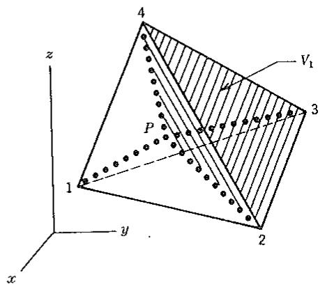
Volume Coordinates. Volume coordinates for a tetrahedron are a direct extension of area coordinates for a triangle, so we will be brief.
text_image
z
4
V₁
3
P
1
y
2
x
Figure 5.2-2. Tetrahedron 1–2–3–4. Volume $V_{1}$ refers to subtetrahedron P–2–3–4, which is identified by hatching.
Point P is the common vertex of four subtetrahedra (Fig. 5.2-2). Volume coordinates are $\xi_{i}=V_{i}/V$ , where the volume of tetrahedron 1–2–3–4 is $V=\Sigma V_{i}$ and i runs from 1 to 4. Cartesian and volume coordinates have the relation
$$
\left\{ \begin{array}{l} 1 \\ x \\ y \\ z \end{array} \right\} = \left[ \begin{array}{c c c c} 1 & 1 & 1 & 1 \\ x _ {1} & x _ {2} & x _ {3} & x _ {4} \\ y _ {1} & y _ {2} & y _ {3} & y _ {4} \\ z _ {1} & z _ {2} & z _ {3} & z _ {4} \end{array} \right] \left\{ \begin{array}{l} \xi_ {1} \\ \xi_ {2} \\ \xi_ {3} \\ \xi_ {4} \end{array} \right\} \tag {5.2-11}
$$
The determinant of the square matrix is $6V$ , where $V$ is positive if nodes are numbered so that the sequence 1-2-3 runs counterclockwise when viewed from node 4. Relations analogous to Eqs. 5.2-7 contain terms from the inverse of the square matrix in Eq. 5.2-11.
The integration formula in volume coordinates is
$$
\int_ {V} \xi_ {1} ^ {k} \xi_ {2} ^ {\ell} \xi_ {3} ^ {m} \xi_ {4} ^ {n} d V = 6 V \frac {k ! \ell ! m ! n !}{(3 + k + \ell + m + n) !} \tag {5.2-12}
$$
A formula analogous to Eq. 5.2-9, but for a special case, is
$$
\int_ {V} x ^ {r} y ^ {s} z ^ {t} d V = \frac {V}{2 0} \sum_ {i = 1} ^ {4} x _ {i} ^ {r} y _ {i} ^ {s} z _ {i} ^ {t} \quad (\text { if } r + s + t = 2) \tag {5.2-13}
$$
provided that the centroid of the tetrahedron is at $x = y = z = 0$ .
Remarks. Triangles and tetrahedra are instances of a simplex, which is a figure in $n$ -dimensional space that has $n + 1$ vertices and is bounded by $n + 1$ surfaces of dimensionality $n - 1$ . Other names for area coordinates are areal, triangular, and trilinear coordinates. Volume coordinates may also be called tetrahedronal coordinates. Area and volume coordinates are known to mathematicians as simplex or barycentric coordinates. They are not new [5.2,5.3] but seem to have been independently devised when finite element theory found a need for them.
# 5.3 INTERPOLATION FIELDS FOR PLANE TRIANGLES
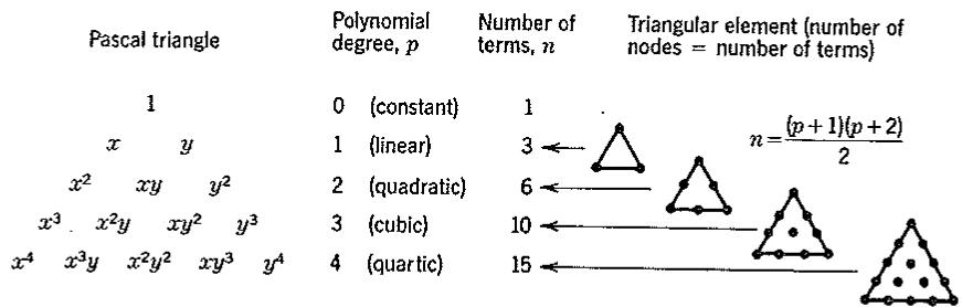
Triangular elements allow a complete polynomial in Cartesian coordinates to be used for the field quantity (e.g., for temperature or for displacement). In other words, in Fig. 5.3-1, with internal nodes present for cubic and higher-order elements, all terms of a truncated Pascal triangle are used in the shape functions: through the second row for a linear element, through the third row for a quadratic element, and so on.
In order to generate finite elements, we seek shape functions $N_{i} = N_{i}(\xi_{1}, \xi_{2}, \xi_{3})$ in the relation $\phi = \Sigma N_{i}\phi_{i}$ , where the $\phi_{i}$ are nodal d.o.f. One way to generate shape functions $N_{i}$ is the usual way of starting with a polynomial that contains constants $a_{i}$ that must be determined. Consider a function $\phi = \phi(\xi_{1}, \xi_{2}, \xi_{3}) = \phi(x, y)$ , where $\phi$ is given by the expansion
$$
\phi = \sum_ {i = 1} ^ {n} a _ {i} \xi_ {1} ^ {q} \xi_ {2} ^ {r} \xi_ {3} ^ {s} \tag {5.3-1}
$$
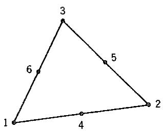
in which q, r, and s are nonnegative integers that range over the n possible combinations for which $q + r + s = p$ . Thus $\phi$ is a complete polynomial of degree p in Cartesian coordinates [5.4]. For example, for the quadratic triangle in Fig. 5.3-2b, n = 6, p = 2, and
$$
\phi = a _ {1} \xi_ {1} ^ {2} + a _ {2} \xi_ {2} ^ {2} + a _ {3} \xi_ {3} ^ {2} + a _ {4} \xi_ {1} \xi_ {2} + a _ {5} \xi_ {2} \xi_ {3} + a _ {6} \xi_ {3} \xi_ {1} \tag {5.3-2}
$$
which, for a straight-sided triangle, is equivalent to
$$
\phi = b _ {1} + b _ {2} x + b _ {3} y + b _ {4} x ^ {2} + b _ {5} x y + b _ {6} y ^ {2} \tag {5.3-3}
$$
where the $b_{i}$ are constants related to constants $a_{i}$ of Eq. 5.3-2.
To obtain shape functions $N_{i}$ from Eq. 5.3-1, we express the $a_{i}$ in terms of nodal d.o.f. $\phi_{i}$ . Consider again the quadratic triangle. Side node 4 is at $\xi_{1} = \xi_{2} = \frac{1}{2}$ and $\xi_{3} = 0$ , side node 5 is at $\xi_{2} = \xi_{3} = \frac{1}{2}$ and $\xi_{1} = 0$ , and side node 6 is at $\xi_{3} = \xi_{1} = \frac{1}{2}$ and $\xi_{2} = 0$ . In Eq. 5.3-2 we set $\phi = \phi_{1}$ for $\xi_{1} = 1$ and $\xi_{2} = \xi_{3} = 0$ , $\phi = \phi_{2}$ for $\xi_{2} = 1$ and $\xi_{3} = \xi_{1} = 0$ , and so on through $\phi = \phi_{6}$ for $\xi_{3} = \xi_{1} = \frac{1}{2}$ and $\xi_{2} = 0$ . After we have solved for the $a_{i}$ , the coefficients of the $\phi_{i}$ are identified as shape functions.
text_image
Pascal triangle
Polynomial
degree, p
Number of
terms, n
Triangular element (number of
nodes = number of terms)
1
x y
x² xy y²
x³ x²y xy² y³
x⁴ x³y x²y² xy³ y⁴
0 (constant)
1 (linear)
2 (quadratic)
3 (cubic)
4 (quartic)
1
3 ←
6 ←
10 ←
15 ←
n=(p+1)(p+2)/2
Figure 5.3-1. Relation between type of plane triangular element and number of polynomial coefficients used for interpolation.
text_image
3
1
2
(a)
text_image
1
2
3
4
5
6
(b)
text_image
3
7
8
9
10
1
4
5
2
(c)
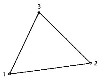
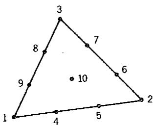
Figure 5.3-2. Triangular elements. (a) Linear. (b) Quadratic. (c) Cubic. Node 10 is at the centroid, $\xi_{1} = \xi_{2} = \xi_{3} = \frac{1}{3}$ .
An alternative way of determining the shape functions is available. With nodes permitted in the element interior, but no derivative d.o.f. permitted at any node, the elements can be identified as Lagrangian. Hence, the Lagrange interpolation formula produces shape functions $N_{i}$ directly. The procedure is not difficult but cannot be explained briefly. Details appear in [5.4].
Shape functions for the elements of Fig. 5.3-2 are as follows. Note that (as expected) each $N_{i}$ is unity at node $i$ but vanishes at all other nodes. For the linear triangle, Fig. 5.3-2a,
$$
N _ {1} = \xi_ {1} \quad N _ {2} = \xi_ {2} \quad N _ {3} = \xi_ {3} \tag {5.3-4}
$$
Thus, individual shape functions of a linear triangle are the area coordinates themselves. For the quadratic triangle, Fig. 5.3-2b,
$$
N _ {1} = \xi_ {1} \left(2 \xi_ {1} - 1\right) \quad N _ {2} = \xi_ {2} \left(2 \xi_ {2} - 1\right) \quad N _ {3} = \xi_ {3} \left(2 \xi_ {3} - 1\right) \tag {5.3-5}
$$
$$
N _ {4} = 4 \xi_ {1} \xi_ {2} \quad N _ {5} = 4 \xi_ {2} \xi_ {3} \quad N _ {6} = 4 \xi_ {3} \xi_ {1}
$$
For the cubic triangle, Fig. 5.3-2c,
$$
N _ {i} = \frac {1}{2} \xi_ {i} (3 \xi_ {i} - 1) (3 \xi_ {i} - 2) \quad \text { for } i = 1, 2, 3
$$
$$
N _ {4} = \frac {9}{2} \xi_ {2} \xi_ {1} (3 \xi_ {1} - 1) \quad N _ {6} = \frac {9}{2} \xi_ {3} \xi_ {2} (3 \xi_ {2} - 1) \tag {5.3-6}
$$
$$
N _ {8} = \frac {9}{2} \xi_ {1} \xi_ {3} (3 \xi_ {3} - 1) \quad N _ {1 0} = 2 7 \xi_ {1} \xi_ {2} \xi_ {3}
$$
and $N_5, N_7$ , and $N_9$ are obtained from $N_4, N_6$ , and $N_8$ , respectively, by interchanging subscripts; for example, $N_5 = 9\xi_1\xi_2(3\xi_2 - 1)/2$ .
Equations 5.3-5 and 5.3-6 can also be used for triangular elements having curved sides. The procedure is described in Section 6.8.
# 5.4 THE LINEAR TRIANGLE
Scalar Field Element. For simplicity, we begin with a scalar field problem. Each node has a single d.o.f. An example application is heat conduction, for which $\phi$ represents temperature (see Section 3.10 or Chapter 16). For the three-node triangle, from Eq. 5.3-4,
$$
\phi = \lfloor \mathrm{N} \rfloor \left\{ \begin{array}{l} \phi_ {1} \\ \phi_ {2} \\ \phi_ {3} \end{array} \right\}, \quad \text { where } \quad \lfloor \mathrm{N} \rfloor = \left\lfloor \xi_ {1} \quad \xi_ {2} \quad \xi_ {3} \right\rfloor \tag {5.4-1}
$$
In order to generate the characteristic matrix [k], derivatives of $\phi$ with respect to $x$ and $y$ are needed. Using Eqs. 5.2-6 and 5.4-1, we have
$$
\frac {\partial \phi}{\partial x} = \sum_ {i = 1} ^ {3} \frac {\partial N _ {i}}{\partial x} \phi_ {i} = \sum_ {i = 1} ^ {3} \frac {\partial \xi_ {i}}{\partial x} \phi_ {i} \tag {5.4-2}
$$
and similarly for $\partial \phi / \partial y$ , where derivatives $\partial \xi_i / \partial x$ and $\partial \xi_i / \partial y$ are given by Eqs. 5.2-7. Hence,
$$
\left\{ \begin{array}{l} \phi_ {, x} \\ \phi_ {, y} \end{array} \right\} = \left[ \begin{array}{l} \mathrm{N} _ {, x} \\ \mathrm{N} _ {, y} \end{array} \right] \left\{ \begin{array}{l} \phi_ {1} \\ \phi_ {2} \\ \phi_ {3} \end{array} \right\} = [ \mathbf {B} ] \left\{ \begin{array}{l} \phi_ {1} \\ \phi_ {2} \\ \phi_ {3} \end{array} \right\}, \quad \text { where } \quad [ \mathbf {B} ] = \frac {1}{2 A} \left[ \begin{array}{l l l} y _ {2 3} & y _ {3 1} & y _ {1 2} \\ x _ {3 2} & x _ {1 3} & x _ {2 1} \end{array} \right] \tag {5.4-3}
$$
and $A$ is the area of the triangle. The element characteristic matrix is
$$
[ \mathbf {k} ] = \int_ {V _ {e}} [ \mathbf {B} ] ^ {T} k [ \mathbf {B} ] d V \tag {5.4-4}
$$
where $k$ is a material property. If $k$ and element thickness $t$ are constant over the element, then $[\mathbf{k}] = ktA[\mathbf{B}]^T[\mathbf{B}]$ .
Constant-Strain Triangle. In plane stress analysis the manipulations are quite similar to those presented in Eqs. 5.4-1 to 5.4-4. Displacement fields $u = u(x,y)$ and $v = v(x,y)$ are each interpolated from nodal d.o.f. $u_i$ and $v_i$ . The linear element has six displacements in the vector of nodal d.o.f. $\{\mathbf{d}\}$ . With $\{\mathbf{d}\} = \left[u_1 \quad v_1 \quad u_2 \quad v_2 \quad u_3 \quad v_3\right]^T$ ,
$$
\left\{ \begin{array}{l} u \\ v \end{array} \right\} = [ \mathrm{N} ] \{\mathbf {d} \}, \quad \text { where } \quad [ \mathrm{N} ] = \left[ \begin{array}{c c c c c c} \xi_ {1} & 0 & \xi_ {2} & 0 & \xi_ {3} & 0 \\ 0 & \xi_ {1} & 0 & \xi_ {2} & 0 & \xi_ {3} \end{array} \right] \tag {5.4-5}
$$
Strains $\{\pmb{\epsilon}\} = [\mathbf{B}]\{\mathbf{d}\}$ are given by Eqs. 1.5-6 and 1.5-8. Using these equations, and also Eqs. 5.2-6 and 5.2-7, we obtain
$$
[ \mathbf {B} ] = [ \partial ] [ \mathbf {N} ] = \frac {1}{2 A} \left[ \begin{array}{c c c c c c} y _ {2 3} & 0 & y _ {3 1} & 0 & y _ {1 2} & 0 \\ 0 & x _ {3 2} & 0 & x _ {1 3} & 0 & x _ {2 1} \\ x _ {3 2} & y _ {2 3} & x _ {1 3} & y _ {3 1} & x _ {2 1} & y _ {1 2} \end{array} \right] \tag {5.4-6}
$$
With [E] given by Eq. 1.7-4 or Eq. 1.7-5, the stiffness matrix of the linear triangle is
$$
[ \mathbf {k} ] = \int_ {V _ {e}} [ \mathbf {B} ] ^ {T} [ \mathbf {E} ] [ \mathbf {B} ] d V \tag {5.4-7}
$$
text_image
y,v
l
l
2
x,u
3
1
c
c
M
M
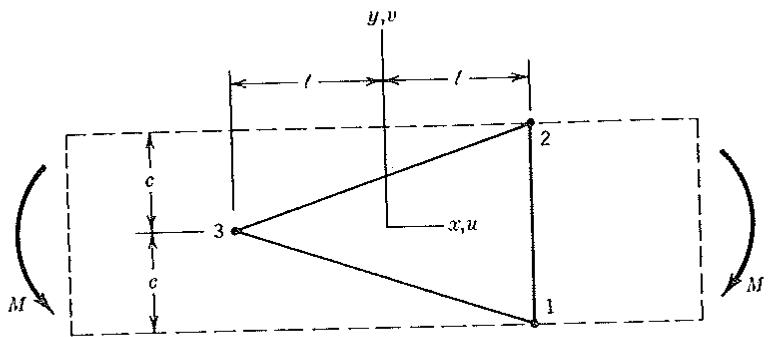
Figure 5.4-1. A linear triangle in a beam subjected to pure bending.
If [E] and element thickness $t$ are constant, then $[\mathbf{k}] = tA[\mathbf{B}]^T [\mathbf{E}][\mathbf{B}]$ .
The element associated with Eq. 5.4-5 is called the constant-strain triangle (CST) because its strain field contains only constants. Because $x$ and $y$ terms are absent, the CST element behaves poorly in bending. Consider, for example, Fig. 5.4-1. Let the origin $x = y = 0$ be motionless, and let bending moment $M$ be of such magnitude that $u = \overline{u}$ at $x = \ell$ on top of the beam. Hence, the correct displacement field associated with pure bending, and the resulting strain field, are
$$
u = \frac {\bar {u}}{c \ell} x y \quad v = \frac {\bar {u}}{2 c \ell} (- x ^ {2} - \nu y ^ {2}) \tag {5.4-8}
$$
$$
\epsilon_ {x} = \frac {\overline {{{u}}}}{c \ell} y \quad \epsilon_ {y} = - \nu \frac {\overline {{{u}}}}{c \ell} y \quad \gamma_ {x y} = 0
$$
To see how the CST represents these bending strains, we impose on the CST nodal displacements $\{d\}$ consistent with the bending field of Eq. 5.4-8 ( $u_{1} = -\overline{u}$ , $u_{2} = \overline{u}$ , $u_{3} = 0$ , and similar prescriptions of $v_{1}$ , $v_{2}$ , and $v_{3}$ from Eqs. 5.4-8). Hence,
text_image
y,v
← h →
B
v=0.25
E
x
D
h
A
C
4h
text_image
32 linear-strain triangles
160 d.o.f., v_A = 0.998, σ_XB = 0.986
text_image
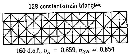
128 constant-strain triangles
160 d.o.f., v_A = 0.859, σ_XB = 0.854
text_image
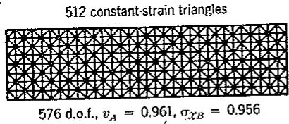
512 constant-strain triangles
576 d.o.f., v_A = 0.961, σ_XB = 0.956
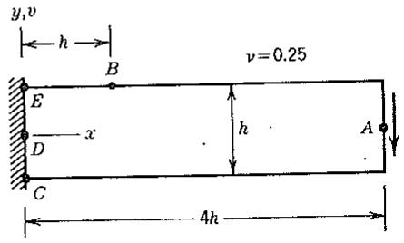
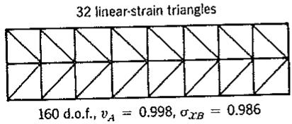
Figure 5.4-2. Tip deflection $v_{A}$ and flexural stress $\sigma_{xB}$ in an isotropic cantilever beam of constant thickness [5.5]. The transverse load is parabolically distributed over the right end. Values reported are ratios of computed values to values predicted by theory of elasticity.
from $\{\pmb{\epsilon}\} = [\mathbf{B}]\{\mathbf{d}\}$ , with [B] given by Eq. 5.4-6, we obtain strains in the CST of Fig. 5.4-1. They are
$$
\epsilon_ {x} = 0 \quad \epsilon_ {y} = 0 \quad \gamma_ {x y} = \left(\frac {1}{c} - \nu \frac {c}{4 \ell^ {2}}\right) \bar {u} \tag {5.4-9}
$$
Clearly these strains are quite wrong. Despite their poor performance in bending, CST elements can adequately model a beam in bending if a great many elements are used through the depth of the beam.
Figure 5.4-2 gives numerical evidence of how the CST behaves. Theoretical values allow for transverse shear deformation and assume that the end at $x = 0$ is free to warp while points $C, D$ , and $E$ remain on a vertical line.
Elements better than the CST are available. Routine use of the CST in stress analysis is not recommended.
# 5.5 THE QUADRATIC TRIANGLE
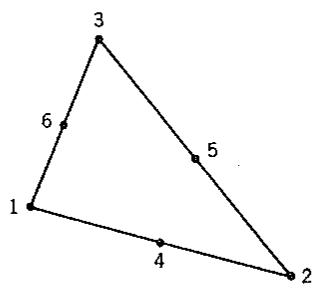
The quadratic triangle with straight sides and midside nodes, Fig. 5.5-1, dates from 1964. It is an excellent element for stress analysis. Its strain field contains a complete linear polynomial for $\epsilon_{x}$ , $\epsilon_{y}$ , and $\gamma_{xy}$ . Accordingly, it is also known as the linear-strain triangle. Its sides can deform into quadratic curves, which means that a uniform edge traction is allocated to nodal loads $\{r_{e}\}$ in the 1–4–1 proportion seen in Fig. 4.3-4.
In the present section we formulate the element stiffness matrix under the restrictions that sides are straight and side nodes are at midsides. In Section 6.8 these restrictions are removed.
For convenience of notation in the following development, we arrange nodal d.o.f. in the order
$$
\{\mathbf {d} \} = \left\lfloor u _ {1} \quad u _ {2} \quad u _ {3} \quad u _ {4} \quad u _ {5} \quad u _ {6} \quad v _ {1} \quad v _ {2} \quad v _ {3} \quad v _ {4} \quad v _ {5} \quad v _ {6} \right] ^ {T} \tag {5.5-1}
$$
The $x$ - and $y$ -direction displacement fields are
$$
u = \sum_ {i = 1} ^ {6} N _ {i} u _ {i} \quad \text { and } \quad v = \sum_ {i = 1} ^ {6} N _ {i} v _ {i} \tag {5.5-2}
$$
text_image
3
6
1
4
5
2
(a)
text_image
φ₂
(b)
text_image
φ₅
(c)
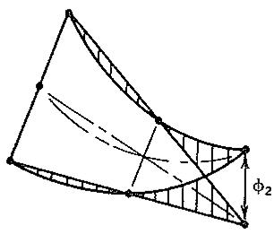
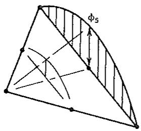
Figure 5.5-1. Quadratic triangle. (a) Node numbering. (b) A vertex-node shape function. (c) A side-node shape function.
where the $N_{i}$ are given by Eqs. 5.3-5. Next
$$
\epsilon_ {x} = \frac {\partial u}{\partial x} = \sum_ {i = 1} ^ {6} \frac {\partial N _ {i}}{\partial x} u _ {i} \quad \text { and } \quad \frac {\partial N _ {i}}{\partial x} = \sum_ {j = 1} ^ {3} \frac {\partial N _ {i}}{\partial \xi_ {j}} \frac {\partial \xi_ {j}}{\partial x} \tag {5.5-3}
$$
where the latter equation is a restatement of Eq. 5.2-6a. Thus, from Eqs. 5.2-7a, 5.3-5, and 5.5-3,
$$
\begin{array}{l} \epsilon_ {x} = \frac {1}{2 A} \left[ (4 \xi_ {1} - 1) y _ {2 3} \quad (4 \xi_ {2} - 1) y _ {3 1} \quad (4 \xi_ {3} - 1) y _ {1 2} \right. \tag {5.5-4} \\ 4 \left(\xi_ {2} y _ {2 3} + \xi_ {1} \dot {y} _ {3 1}\right) \quad 4 \left(\xi_ {3} y _ {3 1} + \xi_ {2} y _ {1 2}\right) \quad 4 \left(\xi_ {1} y _ {1 2} + \xi_ {3} y _ {2 3}\right) \Bigg \} \left\{ \begin{array}{l} u _ {1} \\ u _ {2} \\ u _ {3} \\ u _ {4} \\ u _ {5} \\ u _ {6} \end{array} \right\} \\ \end{array}
$$
Expressions for strains $\epsilon_{y}$ and $\gamma_{xy}$ are developed similarly. The complete result is
$$
\{\epsilon \} = \left\{ \begin{array}{l} \epsilon_ {x} \\ \epsilon_ {y} \\ \gamma_ {x y} \end{array} \right\} = [ \mathbf {B} ] \{\mathbf {d} \}, \quad \text { where } \quad \left[ \mathbf {B} \right] _ {3 \times 1 2} = \left[ \begin{array}{l l} \mathbf {B} _ {x} & \mathbf {0} \\ \mathbf {0} & \mathbf {B} _ {y} \\ \mathbf {B} _ {y} & \mathbf {B} _ {x} \end{array} \right] \tag {5.5-5}
$$
$\mathbf{B}_y$ is the row matrix in Eq. 5.5-4 and $\mathbf{B}_y$ is a similar row matrix.
$B_{x}$ is the row matrix in Eq. 5.5.1 and by $\epsilon$ . Because each strain in $\{\epsilon\}$ is a complete linear field, the following convenient trick can be used [5.5]. We interpolate strains $\{\epsilon\}$ from strains $\{\epsilon_{c}\}$ at corner nodes 1, 2, and 3,
$$
\{\boldsymbol {\epsilon} \} = [ \mathbf {Q} ] \{\boldsymbol {\epsilon} _ {c} \} = [ \mathbf {Q} ] \left[ \begin{array}{l l l l l l l l l} \epsilon_ {x 1} & \epsilon_ {x 2} & \epsilon_ {x 3} & \epsilon_ {y 1} & \epsilon_ {y 2} & \epsilon_ {y 3} & \gamma_ {x y 1} & \gamma_ {x y 2} & \gamma_ {x y 3} \end{array} \right] ^ {T} \tag {5.5-6}
$$
where $\epsilon_{x1}$ is $\epsilon_x$ at node 1, and so on, and, making use of Eq. 5.3-4,
$$
[ \mathbf {Q} ] = \left[ \begin{array}{c c c c c c c c c} \xi_ {1} & \xi_ {2} & \xi_ {3} & 0 & 0 & 0 & 0 & 0 & 0 \\ 0 & 0 & 0 & \xi_ {1} & \xi_ {2} & \xi_ {3} & 0 & 0 & 0 \\ 0 & 0 & 0 & 0 & 0 & 0 & \xi_ {1} & \xi_ {2} & \xi_ {3} \end{array} \right] \tag {5.5-7}
$$
Corner strains $\{\epsilon_c\}$ are written in terms of nodal d.o.f. $\{\mathbf{d}\}$ by evaluating Eq. 5.5-5 at nodes 1, 2, and 3. Thus
$$
\{\epsilon_ {c} \} = [ \mathbf {H} ] \{\mathbf {d} \} \quad \text { and } \quad \{\epsilon \} = [ \mathbf {Q} ] [ \mathbf {H} ] \{\mathbf {d} \} \tag {5.5-8}
$$
where [H] is a 9 by 12 matrix of element dimensions: $H_{11} = 3y_{23} / 2A$ , $H_{12} = -y_{31} / 2A$ , and so on. Combining Eqs. 5.5-6 and 5.5-8, we obtain
$$
\{\epsilon \} = [ \mathbf {B} ] \{\mathbf {d} \}, \quad \text { where } \quad \underset {3 \times 1 2} {[ \mathbf {B} ]} = \underset {3 \times 9} {[ \mathbf {Q} ]} \underset {9 \times 1 2} {[ \mathbf {H} ]} \tag {5.5-9}
$$
The element stiffness matrix is
text_image
4
10
8
9
3
7
6
1
5
2
| Node | 1 | 2 | 3 | 4 | 5 | 6 | 7 | 8 | 9 | 10 |
| $\xi_1$ | 1 | 0 | 0 | 0 | $\frac{1}{2}$ | 0 | $\frac{1}{2}$ | $\frac{1}{2}$ | 0 | 0 |
| $\xi_2$ | 0 | 1 | 0 | 0 | $\frac{1}{2}$ | $\frac{1}{2}$ | 0 | 0 | $\frac{1}{2}$ | 0 |
| $\xi_3$ | 0 | 0 | 1 | 0 | 0 | $\frac{1}{2}$ | $\frac{1}{2}$ | 0 | 0 | $\frac{1}{2}$ |
| $\xi_4$ | 0 | 0 | 0 | 1 | 0 | 0 | 0 | $\frac{1}{2}$ | $\frac{1}{2}$ | $\frac{1}{2}$ |
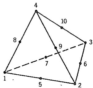
Figure 5.6-1. The quadratic tetrahedron.
$$
[ \mathbf {k} ] = \int_ {V _ {e}} [ \mathbf {B} ] ^ {T} [ \mathbf {E} ] [ \mathbf {B} ] d V = [ \mathbf {H} ] ^ {T} \int_ {V _ {e}} [ \mathbf {Q} ] ^ {T} [ \mathbf {E} ] [ \mathbf {Q} ] d V [ \mathbf {H} ] \tag {5.5-10}
$$
where $dV = t \, dA$ and $t$ is the element thickness. Again, note the ordering of nodal d.o.f. assumed in Eq. 5.5-1. The latter form of Eq. 5.5-10 can be used to advantage in programming. If $t$ is constant or a polynomial in area coordinates, integrations are easily done by means of Eq. 5.2-8.
Behaviors of the constant- and linear-strain triangles are compared in Fig. 5.4-2. We see that the linear-strain triangle is much better in this problem despite using fewer d.o.f.
Fortran coding for straight-sided quadratic triangles of constant thickness may be found in [5.5]. Alternative compact coding for linear, quadratic, and cubic triangles is discussed in [5.6].
# 5.6 THE QUADRATIC TETRAHEDRON
Tetrahedral elements are a straightforward extension of triangular elements. Accordingly, we cite only the quadratic element, Fig. 5.6-1, whose shape functions are
$$
N _ {i} = \xi_ {i} (2 \xi_ {i} - 1) \quad \text { for } i = 1, 2, 3, 4
$$
$$
N _ {5} = 4 \xi_ {1} \xi_ {2} \quad N _ {6} = 4 \xi_ {2} \xi_ {3} \quad N _ {7} = 4 \xi_ {3} \xi_ {1} \tag {5.6-1}
$$
$$
N _ {8} = 4 \xi_ {1} \xi_ {4} \quad N _ {9} = 4 \xi_ {2} \xi_ {4} \quad N _ {1 0} = 4 \xi_ {3} \xi_ {4}
$$
Equation 5.5-10 again describes the element stiffness matrix, where $[k]$ is now 30 by 30, $[E]$ is 6 by 6, and $[B]$ is 6 by 30.
# PROBLEMS
# Section 5.1
5.1 (a) Derive Eq. 5.1-6 by using the substitution procedure suggested below that equation.
(b) Similarly, derive shape functions for cubic interpolation along a line. Nodes are at $\xi_{1} = 1$ , $\xi_{1} = \frac{2}{3}$ , $\xi_{1} = \frac{1}{3}$ , and $\xi_{1} = 0$ . Start with $\phi = a_{1}\xi_{1}^{3} + a_{2}\xi_{1}^{2}\xi_{2} + a_{3}\xi_{1}\xi_{2}^{2} + a_{4}\xi_{2}^{3}$ .
5.2 Use Eq. 5.1-10 to integrate the following functions over span $L$ in Fig. 5.1-1.
(a) $x^{2}$
(b) $\xi_{1}^{3}\xi_{2}^{2}$
(c) $\xi_1x$
5.3 In Eq. 5.1-9, let $A$ vary linearly from $A_1$ at node 1 to $A_2$ at node 2. Determine the resulting stiffness matrix [k].
5.4 In Eq. 5.1-6, let $\phi$ represent axial displacement $u$ of a uniform bar element. Determine the 3 by 3 element stiffness matrix. Let node 3 lie at the center of the bar (hence, $\xi_{1}$ and $\xi_{2}$ are linear functions of $x$ ).
# Section 5.2
5.5 Let $x_{1}$ and $y_{1}$ in [A] of Eq. 5.2-4 be replaced by $x$ and $y$ . Then, Eq. 5.2-5 yields $2A_{1} = \det[A]$ . Similar expressions for $2A_{2}$ and $2A_{3}$ can be written. Hence, $\left|\xi_{1} \xi_{2} \xi_{3}\right|^{T} = \left[2A_{1} 2A_{2} 2A_{3}\right]^{T} / 2A = [A]^{-1}\left[1 x y\right]^{T}$ . In this way verify the expression for $[A]^{-1}$ in Eq. 5.2-4.
5.6 (a) Verify that $[\mathbf{A}]^{-1}$ is correctly stated in Eq. 5.2-4 by forming the product $[\mathbf{A}][\mathbf{A}]^{-1}$ .
(b) Show that the equation of side 1 of the triangle is $x_{2}y_{3} - x_{3}y_{2} + y_{23}x + x_{32}y = 0$ .
(c) Derive the latter expression for 2A in Eq. 5.2-5 from det[A].
(d) In Fig. 5.2-1, drop lines from the triangle vertices to the $x$ axis. One can now identify three trapezoids, whose upper sides are 1-2, 2-3, and 3-1. Two trapezoidal areas minus a third equals the triangle area. Hence, derive the expression $2A = x_{21}y_{31} - x_{31}y_{21}$ in Eq. 5.2-5.
(e) Is it also true that $2A = x_{32}y_{12} - x_{12}y_{32}$ ? Explain.
5.7 Let the function $\phi = 27\xi_1\xi_2\xi_3$ be defined over the triangle in Fig. 5.2-1.
(a) Sketch this function in isometric view (analogous to Fig. 1.1-3).
(b) Integrate $\phi$ over the triangle area $A$ .
5.8 Let a function $\phi$ vary linearly over face 1-2-3 of a tetrahedron. Values of $\phi$ at corner nodes on this face are $\phi_1, \phi_2$ , and $\phi_3$ . The integral of $\phi$ over face 1-2-3 is $A_{123}(\phi_1 + \phi_2 + \phi_3)/3$ . Derive this result by formal integration.
5.9 Show that Eq. 5.2-10 is produced by Eq. 5.2-8.
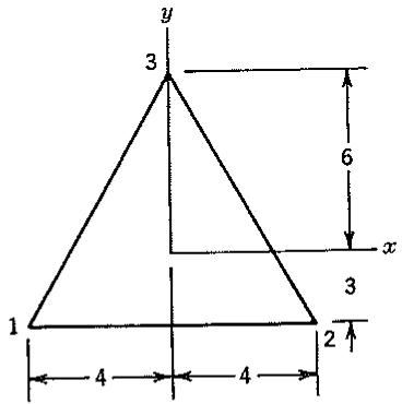
5.10 For a triangle having the dimensions shown, use formulas for area moments and products of inertia to numerically verify Eq. 5.2-9 for the case $r + s = 2$ .
text_image
y
3
6
x
1
3
2
4
4
Problem 5.10