5.11 For $r + s = 1$ and again for $r + s = 2$ , write integration formulas analogous to Eq. 5.2-9 if the origin of coordinates need not be at the centroid of the triangle. (Let the centroid have coordinates $x = x_{c}$ and $y = y_{c}$ .) # Section 5.3 5.12 For a cubic triangle (10 nodes), write an equation analogous to Eq. 5.3-2. 5.13 From Eq. 5.3-2, derive the shape functions of Eqs. 5.3-5. # Section 5.4 5.14 (a) For a linear triangle, the equation that corresponds to Eq. 5.3-3 is $\phi = b_{1} + b_{2}x + b_{3}y$ . From this, and without using area coordinates, obtain shape functions $N_{1}, N_{2}$ , and $N_{3}$ in terms of $x, y$ , and Cartesian coordinates $x_{i}$ and $y_{i}$ of the vertex nodes. (b) Show that the $N_{i}$ of part (a) yield the $N_{i}$ of Eq. 5.3-4. (c) Obtain [B] of Eq. 5.4-6 from the $N_{i}$ of part (a). 5.15 Verify the results given in Eqs. 5.4-9. Start with Eqs. 5.4-8. # Section 5.5 5.16 Write out the first three rows of matrix [H] in Eq. 5.5-8. Then show that the product [Q][H] in Eq. 5.5-9 yields the row matrix $\mathbf{B}_x$ defined by Eq. 5.5-4 (check at least the first row of the product). 5.17 Consider use of the quadratic triangle for a scalar field problem (similar to Eqs. 5.4-1 through 5.4-3 for the linear triangle). Redefine matrices [Q] and [H] of the quadratic triangle as may be necessary in order to obtain a result for a scalar field problem analogous to the latter form of Eq. 5.5-10. If material property $k$ and thickness $t$ are constant, determine $c$ and [M] in the form $[\mathbf{k}] = c[\mathbf{H}]^T[\mathbf{M}][\mathbf{H}]$ , where integrations have been completed to yield [M], and $c$ represents constants. 5.18 Impose nodal displacements associated with u and v of Eqs. 5.4-8 on the element of Fig. 5.4-1, but consider that the element is a quadratic triangle (six nodes; Eqs. 5.5-2). For simplicity, consider the special case v = 0. Does the quadratic element display the correct strains? 5.19 Let an edge of a quadratic triangle lie parallel to the $x$ axis. Determine the consistent nodal loads that result from the following distributed loads on this edge. (a) Uniform traction in the $y$ direction. (b) Shear stress parallel to the edge, varying parabolically from a maximum at midedge to zero at the adjacent vertices. (c) A traction in the $y$ direction that varies linearly from $+\overline{\sigma}$ at one vertex to $-\overline{\sigma}$ at the adjacent vertex. 5.20 (a) Evaluate nodal loads $\{\mathbf{r}_e\}$ that result from heating of an isotropic quadratic triangle. Let the temperature vary linearly over the element and be defined by corner temperatures $T_{1}, T_{2}$ , and $T_{3}$ . Express $\{\mathbf{r}_e\}$ in terms of $E$ , $\alpha, \nu$ , and corner coordinates and temperatures. (b) Show that the nodal forces of part (a) are self-equilibrating—that is, show $\Sigma (r_e)_i = 0$ . # Section 5.6 5.21 The strain-displacement relation for a tetrahedron can be written in the form $\{\epsilon\} = [\mathbf{Q}][\mathbf{H}]\{\mathbf{d}\}$ (analogous to Eqs. 5.5-9). Write out matrices [Q] and [H] for a quadratic tetrahedron. Use the symbol $a_{ij}$ to denote coefficients of the inverse of the matrix in Eq. 5.2-11, but do not bother to compute the inverse. 5.22 Let a uniform pressure $p$ act normal to one face of a quadratic tetrahedron. What are the consistent nodal loads? # THE ISOPARAMETRIC FORMULATION The “isoparametric” formulation can be used to produce many types of useful elements. Plane isoparametric elements are emphasized in the present chapter. Numerical integration, used in element formulation, is described and its possible pitfalls are discussed. 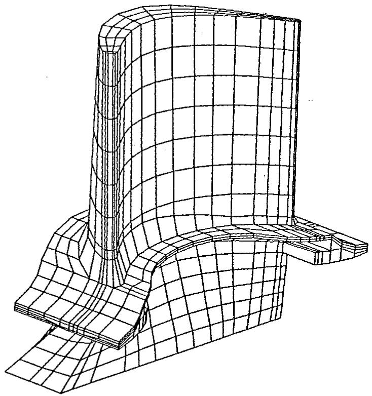# 6.1 INTRODUCTION The isoparametric formulation makes it possible to generate elements that are nonrectangular and have curved sides. These shapes have obvious uses in grading a mesh from coarse to fine, in modeling arbitrary shapes, and in modeling curved boundaries (Fig. 6.1-1). The isoparametric family includes elements for plane, solid, plate, and shell problems. There are also special elements for fracture mechanics and elements for nonstructural problems. 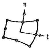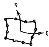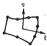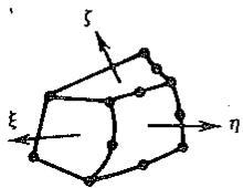In formulating isoparametric elements, natural coordinate systems must be used (systems $\xi\eta$ and $\xi\eta\zeta$ in Fig. 6.1-2). Displacements are expressed in terms of natural 

natural_image

3D wireframe model of a curved structural component with grid pattern (no text or symbols)

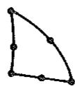
Figure 6.1-1. Turbine blade, modeled by solid elements. (Courtesy of NASA Lewis Research Center, Cleveland, Ohio.)  {a}  (b)  {c}  {d}  {e} Figure 6.1-2. Example isoparametric elements. (a) Quadratic plane element. (b) Cubic plane element. (c) A “degraded” cubic element. The left and lower sides can be joined to linear and quadratic elements. (d) Quadratic solid element with some linear edges. (e) A quadratic plane triangle. coordinates, but must be differentiated with respect to global coordinates $x, y$ , and $z$ . Accordingly, a transformation matrix, called [J], must be invoked. In addition, integrations must be done numerically rather than analytically if elements are nonrectangular. Closed-form integrations are possible in some special cases, but expressions tend to be lengthy, tedious to work out, and therefore more subject to errors of algebra and coding than numerical integration. The term “isoparametric” means “same parameters” and is explained as follows. Because either displacements or coordinates can be interpolated from nodal values, 1. Nodal d.o.f. $\{\mathbf{d}\}$ define displacements $\lfloor u \quad v \quad w \rfloor$ of a point in the element; that is, $\left| u \quad v \quad w \right|^T = [\mathbf{N}]\{\mathbf{d}\}$ . 2. Nodal coordinates $\{\mathbf{c}\}$ define coordinates $\lfloor x\quad y\quad z\rfloor$ of a point in the element; that is, $\lfloor x\quad y\quad z\rfloor^T = [\tilde{\mathbf{N}}]\{\mathbf{c}\}$ . Shape function matrices [N] and [N] are functions of $\xi$ , $\eta$ , and $\zeta$ . An element is isoparametric if [N] and [N] are identical. If [N] is of higher degree than [N], the element is called subparametric, but if [N] is of lower degree than [N], the element is called superparametric. Isoparametric elements were developed by Taig in 1958 [1.10], but no work was published until 1966 [6.1]. 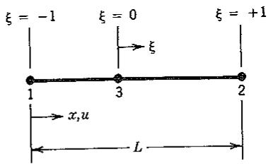# 6.2 AN ISOPARAMETRIC BAR ELEMENT As a simple introduction to isoparametric elements, consider a straight, three-node element, Fig. 6.2-1a. Coordinate $\xi$ is a natural or intrinsic coordinate: ends of the bar lie at $\xi = \pm 1$ , regardless of the physical length $L$ of the bar. Moreover, $\xi$ is attached to the bar and remains an axial coordinate regardless of how the bar 

text_image

ξ = -1 ξ = 0 ξ = +1 1 3 2 x,u L

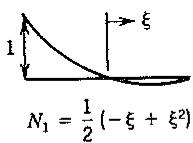
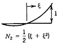
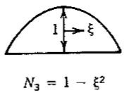
(a)    (b) Figure 6.2-1. (a) Three-node (quadratic) bar element with natural coordinate $\xi$ . (b) The three shape functions. is oriented in global coordinates xyz. For convenience, not necessity, $\xi$ and x are collinear in the present example. Node 3 is at $\xi = 0$ , but need not be at the physical center of the bar. Coordinate $\xi$ in Fig. 6.2-1 differs from the natural coordinates $\xi_{1}$ and $\xi_{2}$ used in Section 5.1; $\xi$ is chosen in preference to $\xi_{1}$ and $\xi_{2}$ because it is more closely related to coordinates $\xi \eta$ used for plane quadrilateral elements in subsequent discussions. We begin with an assumed field, written in terms of the natural coordinate $\xi$ , for both coordinate $x$ and axial displacement $u$ : $$ x = \left\lfloor 1 \quad \xi \quad \xi^ {2} \right\rfloor \left\{ \begin{array}{l} a _ {1} \\ a _ {2} \\ a _ {3} \end{array} \right\} \quad \text { and } \quad u = \left\lfloor 1 \quad \xi \quad \xi^ {2} \right\rfloor \left\{ \begin{array}{l} a _ {4} \\ a _ {5} \\ a _ {6} \end{array} \right\} \tag {6.2-1} $$ where the $a_{i}$ are generalized coordinates. One can now determine shape functions by following the formal substitution procedure detailed in Eqs. 3.8-5 through 3.8-8. Another way to determine shape functions is to use Lagrange's interpolation formula, Eq. 3.12-3, replacing $x$ 's by $\xi$ 's. Or, finally, one can proceed largely by inspection. For example, note that the linear ramps $\frac{1}{2}(1 - \xi)$ and $\frac{1}{2}(1 + \xi)$ have magnitude $\frac{1}{2}$ at $\xi = 0$ (Fig. 3.12-1a). We require that $N_{1}$ and $N_{2}$ both vanish at $\xi = 0$ . Accordingly, if $N_{3} = 1 - \xi^{2}$ is known, we obtain $N_{1} = \frac{1}{2}(1 - \xi) - \frac{1}{2} N_{3}$ and $N_{2} = \frac{1}{2}(1 + \xi) - \frac{1}{2} N_{3}$ . By any of these procedures, we arrive at $$ x = \left\lfloor \mathrm{N} \right\rfloor \left\lfloor x _ {1} \quad x _ {2} \quad x _ {3} \right\rfloor^ {T} \quad \text { and } \quad u = \left\lfloor \mathrm{N} \right\rfloor \left\lfloor u _ {1} \quad u _ {2} \quad u _ {3} \right\rfloor^ {T} \tag {6.2-2} $$ where $$ \lfloor \mathrm{N} \rfloor = \left[ \frac {1}{2} (- \xi + \xi^ {2}) \quad \frac {1}{2} (\xi + \xi^ {2}) \quad 1 - \xi^ {2} \right] \tag {6.2-3} $$ The element is isoparametric because the same $\{N\}$ is used for interpolation of both x and u. To evaluate x or u at any point on the bar, we substitute the $\xi$ coordinate of that point into Eq. 6.2-2. Construction of the element stiffness matrix requires that the strain-displacement relation be known. Axial strain $\epsilon_{x}$ is $$ \epsilon_ {x} = \frac {d u}{d x} = \left(\frac {d}{d x} [ N ]\right) \left\{ \begin{array}{l} u _ {1} \\ u _ {2} \\ u _ {3} \end{array} \right\}, \quad \text { where } \quad \frac {d}{d x} = \frac {d \xi}{d x} \frac {d}{d \xi} \tag {6.2-4} $$ The chain rule for $d / dx$ must be invoked because $\lfloor \mathbf{N} \rfloor$ is expressed in terms of $\xi$ rather than in terms of $x$ . Unfortunately, $d\xi / dx$ is not immediately available. We must first calculate its inverse, $dx / d\xi$ , from the first of Eqs. 6.2-2. Let $J = dx / d\xi$ . Then $$ J = \frac {d}{d \xi} [ N ] \left\{ \begin{array}{l} x _ {1} \\ x _ {2} \\ x _ {3} \end{array} \right\} = \left\lfloor \frac {1}{2} (- 1 + 2 \xi) \quad \frac {1}{2} (1 + 2 \xi) \quad - 2 \xi \right] \left\{ \begin{array}{l} x _ {1} \\ x _ {2} \\ x _ {3} \end{array} \right\} \tag {6.2-5} $$ J is called a Jacobian. It can be regarded as a scale factor that describes the physical length dx associated with a reference length $d\xi$ ; that is, dx = J $d\xi$ . The element stiffness matrix is $$ [ \mathbf {k} ] = \int_ {0} ^ {L} \left\lfloor \mathbf {B} \right] ^ {T} A E \left\lfloor \mathbf {B} \right\rfloor d x = \int_ {- 1} ^ {1} \left\lfloor \mathbf {B} \right] ^ {T} A E \left\lfloor \mathbf {B} \right\rfloor J d \xi \tag {6.2-6} $$ where, from Eqs. 6.2-4 and 6.2-5, $$ \left\lfloor \mathrm{B} \right] = \frac {1}{J} \frac {d}{d \xi} \left\lfloor \mathrm{N} \right] = \frac {1}{J} \left\lfloor \frac {1}{2} (- 1 + 2 \xi) \quad \frac {1}{2} (1 + 2 \xi) \quad - 2 \xi \right\rfloor \tag {6.2-7} $$ Only if node 3 is at the middle of the bar does $J$ reduce to the constant value $J = L / 2$ . The specific form of $J$ depends on the numerical values assigned to $x_{1}$ , $x_{2}$ , and $x_{3}$ in Eq. 6.2-5. In general, $J$ is a function of $\xi$ . Accordingly, $[\mathbf{B}]$ contains $\xi$ in both numerator and denominator of every term. Therefore, Eq. 6.2-6 cannot be conveniently integrated in closed form. In practice, numerical integration is used instead. The preceding example illustrates some of the concepts and manipulations associated with isoparametric elements, but shows none of their versatility. For this we must consider plane and solid elements. # 6.3 PLANE BILINEAR ISOPARAMETRIC ELEMENT The following development generalizes the four-node element of Fig. 4.2-4 from a rectangle to arbitrary quadrilateral shape. For a rectangular element of side lengths $2a$ and $2b$ , with $x = 0$ and $y = 0$ at the element center, isoparametric coordinates $\xi$ and $\eta$ can be regarded as dimensionless Cartesian coordinates $\xi = x/a$ and $\eta = y/b$ . This special case can be used as a study aid in the following discussion. 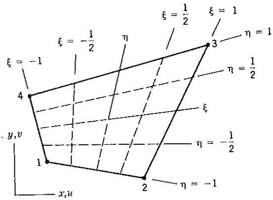Isoparametric coordinates in a plane are shown in Fig. 6.3-1a. For a four-node element, axes $\xi$ and $\eta$ pass through midpoints of opposite sides. Axes $\xi$ and $\eta$ need not be orthogonal, and neither need be parallel to the $x$ axis or the $y$ axis. Sides of the element are at $\xi = \pm 1$ and at $\eta = \pm 1$ . Coordinates $x$ and $y$ within the element are defined by 

text_image

ξ = -1 ξ = -1/2 η ξ = 1/2 ξ = 1 η = 1 3 η = 1/2 y, v ξ η = -1/2 1 2 η = -1 x, u

(a) 

text_image

η ← 1 → ← 1 → 4 3 1 2 1 ξ 1

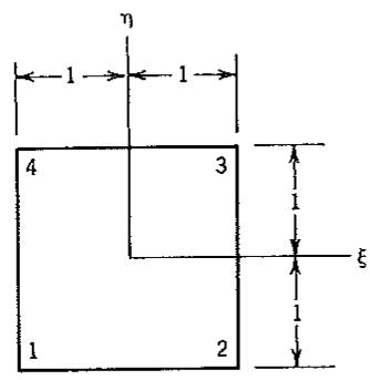
(b) Figure 6.3-1. (a) Four-node plane isoparametric element in $xy$ space. (b) Plane isoparametric element in $\xi \eta$ space. $$ x = \sum N _ {i} x _ {i} \quad \text { and } \quad y = \sum N _ {i} y _ {i} \tag {6.3-1} $$ Summations run from 1 to 4. Individual shape functions are $$ N _ {1} = \frac {1}{4} (1 - \xi) (1 - \eta) \quad N _ {2} = \frac {1}{4} (1 + \xi) (1 - \eta) \tag {6.3-2} $$ $$ N _ {3} = \frac {1}{4} (1 + \xi) (1 + \eta) \quad N _ {4} = \frac {1}{4} (1 - \xi) (1 + \eta) $$ These $N_{i}$ are clearly similar to those in Eq. 3.12-10; indeed they are identical for the special case $\xi = x / a$ and $\eta = y / b$ . Equations 6.3-2 can be established by any of the usual methods: formal substitution, Lagrange's interpolation formula, or inspection and trial. For a given element geometry, the orientation of $\xi \eta$ axes with respect to $xy$ axes is dictated by Eqs. 6.3-2 and the node numbers assigned to the element at hand. For example, in Fig. 6.3-1a, a cyclic change in node numbers (2 changed to 1, 3 changed to 2, etc.) would place the $\xi$ axis where the $\eta$ axis is now shown and would place the $\eta$ axis in the present $-\xi$ direction. Figure 6.3-1b would not be changed: because of Eqs. 6.3-2, node 1 is always at $\xi = \eta = -1$ , node 2 always at $\xi = 1$ and $\eta = -1$ , and so on. The point $\xi = \eta = 0$ can be regarded as the center of the element, but it is not in general the centroid of the element area. Scalar Field Element. Let the field quantity be $\phi$ , where $\phi = \phi(x,y)$ or $\phi = \phi(\xi,\eta)$ . For example, in heat conduction analysis, $\phi$ represents temperature. The simplest element has one d.o.f. per node. Within a four-node element, $\phi$ is interpolated from nodal values $\{\phi_e\} = \lfloor \phi_1 \quad \phi_2 \quad \phi_3 \quad \phi_4 \rfloor^T$ , $$ \phi = \lfloor \mathrm{N} \rfloor \left\{\phi_ {e} \right\} \quad \text { or } \quad \phi = \sum N _ {i} \phi_ {i} \tag {6.3-3} $$ where, to make the element isoparametric, the $N_{i}$ are taken from Eq. 6.3-2. The following derivatives of $\phi$ are needed in element formulation: $$ \left\{ \begin{array}{l} \phi_ {, x} \\ \phi_ {, y} \end{array} \right\} = [ \mathbf {B} ] \left\{\phi_ {e} \right\}, \quad \text { where } \quad [ \mathbf {B} ] = \left[ \begin{array}{c c c c} N _ {1, x} & N _ {2, x} & N _ {3, x} & N _ {4, x} \\ N _ {1, y} & N _ {2, y} & N _ {3, y} & N _ {4, y} \end{array} \right] \tag {6.3-4} $$ For the element characteristic matrix we refer to Eq. 3.10-9. With k a material property and t the element thickness, $$ [ \mathbf {k} ] = \int \int [ \mathbf {B} ] ^ {T} k [ \mathbf {B} ] t d x d y = \int_ {- 1} ^ {1} \int_ {- 1} ^ {1} [ \mathbf {B} ] ^ {T} k [ \mathbf {B} ] t J d \xi d \eta \tag {6.3-5} $$ in which J arises because of the change of coordinates. $^{1}$ In the latter form of Eq. 6.3-5, [B] is a function of $\xi$ and $\eta$ , and is determined as follows. Because $\phi$ is expressed in terms of $\xi$ and $\eta$ , not $x$ and $y$ , derivatives needed in Eq. 6.3-4 are not immediately available. We therefore begin by taking derivatives with respect to $\xi$ and $\eta$ instead: $$ \left\{ \begin{array}{l} \phi_ {, \xi} \\ \phi_ {, \eta} \end{array} \right\} = [ \mathbf {D} _ {N} ] \left\{\phi_ {e} \right\}, \quad \text { where } \quad [ \mathbf {D} _ {N} ] = \left[ \begin{array}{c c c c} N _ {1, \xi} & N _ {2, \xi} & N _ {3, \xi} & N _ {4, \xi} \\ N _ {1, \eta} & N _ {2, \eta} & N _ {3, \eta} & N _ {4, \eta} \end{array} \right] \tag {6.3-6} $$ From Eqs. 6.3-2, $N_{1,\xi} = -(1 - \eta)/4$ , $N_{1,\eta} = -(1 - \xi)/4$ , and so on. Next we must relate $\phi_{, \xi}$ and $\phi_{, \eta}$ to $\phi_{, x}$ and $\phi_{, y}$ . The necessary relation is derived subsequently and has the form $$ \left\{ \begin{array}{l} \phi_ {, x} \\ \phi_ {, y} \end{array} \right\} = [ \Gamma ] \left\{ \begin{array}{l} \phi_ {, \xi} \\ \phi_ {, \eta} \end{array} \right\} \tag {6.3-7} $$ which provides the [B] matrix as $$ [ \mathbf {B} ] = [ \boldsymbol {\Gamma} ] [ \mathbf {D} _ {N} ] \tag {6.3-8} $$ Jacobian Matrix [J]. We now seek an expression for $[\Gamma]$ in Eq. 6.3-7. By the chain rule, $$ \frac {\partial \phi}{\partial x} = \frac {\partial \phi}{\partial \xi} \frac {\partial \xi}{\partial x} + \frac {\partial \phi}{\partial \eta} \frac {\partial \eta}{\partial x} \quad \text {and} \quad \frac {\partial \phi}{\partial y} = \frac {\partial \phi}{\partial \xi} \frac {\partial \xi}{\partial y} + \frac {\partial \phi}{\partial \eta} \frac {\partial \eta}{\partial y} \tag {6.3-9} $$ Thus $\Gamma_{11} = \xi_{,x}, \Gamma_{12} = \eta_{,x}, \Gamma_{21} = \xi_{,y}$ and $\Gamma_{22} = \eta_{,y}$ . Unfortunately, the partial derivatives of $\xi$ and $\eta$ with respect to $x$ and $y$ are not directly available from our equations. Therefore, we must write the inverse of Eq. 6.3-7 first, which is easily done. We write $$ \begin{array}{l} \frac {\partial \phi}{\partial \xi} = \frac {\partial \phi}{\partial x} \frac {\partial x}{\partial \xi} + \frac {\partial \phi}{\partial y} \frac {\partial y}{\partial \xi} \\ \frac {\partial \phi}{\partial \eta} = \frac {\partial \phi}{\partial x} \frac {\partial x}{\partial \eta} + \frac {\partial \phi}{\partial y} \frac {\partial y}{\partial \eta} \end{array} \quad \text {or} \quad \left\{ \begin{array}{l} \phi , \xi \\ \phi , \eta \end{array} \right\} = [ J ] \left\{ \begin{array}{l} \phi , x \\ \phi , y \end{array} \right\} \tag {6.3-10} $$ where [J] is called the Jacobian matrix: $$ [ \mathbf {J} ] = \left[ \begin{array}{l l} x, _ {\xi} & y, _ {\xi} \\ x, _ {\eta} & y, _ {\eta} \end{array} \right] = \left[ \begin{array}{l l} \sum N _ {i, \xi} x _ {i} & \sum N _ {i, \xi} y _ {i} \\ \sum N _ {i, \eta} x _ {i} & \sum N _ {i, \eta} y _ {i} \end{array} \right] \tag {6.3-11} $$ Equation 6.3-11 is valid for all plane isoparametric elements, where i ranges over the number of nodes (and shape functions) used to define element geometry. For the four-node element at hand, i runs from 1 to 4, so, from Eqs. 6.3-6 and 6.3-11, $$ [ \mathbf {J} ] = [ \mathbf {D} _ {N} ] \left[ \begin{array}{l l} x _ {1} & y _ {1} \\ x _ {2} & y _ {2} \\ x _ {3} & y _ {3} \\ x _ {4} & y _ {4} \end{array} \right] \tag {6.3-12} $$ in which, for the bilinear element, $$ \left[ \mathbf {D} _ {N} \right] = \frac {1}{4} \left[ \begin{array}{c c c c} - (1 - \eta) & (1 - \eta) & (1 + \eta) & - (1 + \eta) \\ - (1 - \xi) & - (1 + \xi) & (1 + \xi) & (1 - \xi) \end{array} \right] \tag {6.3-13} $$ Matrix [Γ] is the inverse of [J], $$ [ \Gamma ] = [ J ] ^ {- 1} = \frac {1}{J} \left[ \begin{array}{c c} J _ {2 2} & - J _ {1 2} \\ - J _ {2 1} & J _ {1 1} \end{array} \right] \tag {6.3-14} $$ where J is the determinant of the Jacobian matrix $$ J = \det [ J ] = J _ {1 1} J _ {2 2} - J _ {2 1} J _ {1 2} \tag {6.3-15} $$ Jacobian J can be regarded as a scale factor that yields area dx dy from $d\xi d\eta$ . In general, J is a function of $\xi$ and $\eta$ , but for rectangles and parallelograms it is constant. All ingredients are now at hand for evaluation of $[k]$ according to the second form of Eqs. 6.3-5. Plane Stress Element. There are now two fields—namely, the displacements $$ u = \sum N _ {i} u _ {i} \quad \text { and } \quad v = \sum N _ {i} v _ {i} \tag {6.3-16} $$ where the $N_{i}$ are again the same as the functions used to define shape, Eqs. 6.3-1 and 6.3-2. Displacements u and v are x-parallel and y-parallel; they are not $\xi$ -parallel and $\eta$ -parallel. The strain-displacement relation is $\{\epsilon\} = [\mathbf{B}]\{\mathbf{d}\}$ , where $\{\mathbf{d}\} = [u_1 v_1 u_2 \cdots v_4]^T$ and [B] is the product of the rectangular matrices in the following three equations, which respectively state the strain-displacement relation (Eq. 1.5-6), an expanded form of Eq. 6.3-7, and an expanded form of Eq. 6.3-6: $$ \{\epsilon \} = \left\{ \begin{array}{l} \epsilon_ {x} \\ \epsilon_ {y} \\ \gamma_ {x y} \end{array} \right\} = \left[ \begin{array}{c c c c} 1 & 0 & 0 & 0 \\ 0 & 0 & 0 & 1 \\ 0 & 1 & 1 & 0 \end{array} \right] \left\{ \begin{array}{l} u _ {, x} \\ u _ {, y} \\ v _ {, x} \\ v _ {, y} \end{array} \right\} \tag {6.3-17} $$ $$ \left\{ \begin{array}{l} u _ {, x} \\ u _ {, y} \\ v _ {, x} \\ v _ {, y} \end{array} \right\} = \left[ \begin{array}{c c c c} \Gamma_ {1 1} & \Gamma_ {1 2} & 0 & 0 \\ \Gamma_ {2 1} & \Gamma_ {2 2} & 0 & 0 \\ 0 & 0 & \Gamma_ {1 1} & \Gamma_ {1 2} \\ 0 & 0 & \Gamma_ {2 1} & \Gamma_ {2 2} \end{array} \right] \left\{ \begin{array}{l} u _ {, \xi} \\ u _ {, \eta} \\ v _ {, \xi} \\ v _ {, \eta} \end{array} \right\} \tag {6.3-18} $$ $$ \left\{ \begin{array}{l} u, _ {\xi} \\ u, _ {\eta} \\ v, _ {\xi} \\ v, _ {\eta} \end{array} \right\} = \left[ \begin{array}{c c c c c c c c} N _ {1, \xi} & 0 & N _ {2, \xi} & 0 & N _ {3, \xi} & 0 & N _ {4, \xi} & 0 \\ N _ {1, \eta} & 0 & N _ {2, \eta} & 0 & N _ {3, \eta} & 0 & N _ {4, \eta} & 0 \\ 0 & N _ {1, \xi} & 0 & N _ {2, \xi} & 0 & N _ {3, \xi} & 0 & N _ {4, \xi} \\ 0 & N _ {1, \eta} & 0 & N _ {2, \eta} & 0 & N _ {3, \eta} & 0 & N _ {4, \eta} \end{array} \right] _ {8 \times 1} ^ {\{\mathbf {d} \}} \tag {6.3-19} $$ Coefficients $\Gamma_{ij}$ are given by Eqs. 6.3-11 and 6.3-14. The element stiffness matrix, Eq. 4.1-5, is $$ [ \mathbf {k} ] _ {8 \times 8} = \int \int_ {8 \times 3} [ \mathbf {B} ] ^ {T} [ \mathbf {E} ] _ {3 \times 3} [ \mathbf {B} ] _ {3 \times 8} t d x d y = \int_ {- 1} ^ {1} \int_ {- 1} ^ {1} [ \mathbf {B} ] ^ {T} [ \mathbf {E} ] [ \mathbf {B} ] t J d \xi d \eta \tag {6.3-20} $$ where t is the element thickness. Contributions to the element load vector $\{r_{e}\}$ , Eq. 4.1-6, include the terms $$ \int_ {- 1} ^ {1} \int_ {- 1} ^ {1} \left([ \mathbf {B} ] ^ {T} [ \mathbf {E} ] \left\{\boldsymbol {\epsilon} _ {0} \right\} - [ \mathbf {B} ] ^ {T} \left\{\boldsymbol {\sigma} _ {0} \right\} + [ \mathbf {N} ] ^ {T} \left\{\mathbf {F} \right\}\right) t J d \xi d \eta \tag {6.3-21} $$ For convenience in computer programming, contributions to $\{r_{e}\}$ from surface tractions $\{\Phi\}$ are evaluated separately. For this, the manipulations associated with isoparametric coordinates may be unnecessary. For example, linearly varying traction on a straight edge is allocated to nodes as shown in Fig. 4.3-3. Remarks. Isoparametric elements are geometrically isotropic. Thus, for the element of Fig. 6.3-1, the numerical values of coefficients in [k] do not depend on whether element nodes are labeled 1-2-3-4, 2-3-4-1, 3-4-1-2, or 4-1-2-3. However, the cyclic order must be maintained and must run counterclockwise if $J$ is not to become negative over part or all of the element. From Eqs. 6.3-8 and 6.3-14 we see that $J$ appears in the denominator of each coefficient $B_{ij}$ . Again, $J$ is in general a function of $\xi$ and $\eta$ . Therefore, the denominator of each term to be integrated in Eqs. 6.3-5 and 6.3-20 will in general contain a polynomial of the form $a_1 + a_2\xi + a_3\eta + a_4\xi\eta$ . (A polynomial of higher degree appears for elements having more than four nodes.) Closed-form expressions for integrals of terms in Eq. 6.3-20 would be lengthy. Accordingly, integration is done numerically instead, usually by formulas known as Gauss quadrature. # 6.4 SUMMARY OF GAUSS QUADRATURE "Quadrature" is the name applied to evaluating an integral numerically, rather than analytically as is done in tables of integrals. There are many quadrature rules. The reader may have encountered the Newton–Cotes rules such as Simpson's rule. Here we discuss only the Gauss rules, as they are most appropriate for elements discussed in this chapter. One Dimension. An integral having arbitrary limits can be transformed so that its limits are from -1 to +1. With $f = f(x)$ , and with the substitution $x = \frac{1}{2}(1 - \xi)x_{1} + \frac{1}{2}(1 + \xi)x_{2}$ , $$ I = \int_ {x _ {1}} ^ {x _ {2}} f d x \quad \text { becomes } \quad I = \int_ {- 1} ^ {1} \phi d \xi \tag {6.4-1} $$ Thus the integrand is changed from $f = f(x)$ to $\phi = \phi(\xi)$ , where $\phi$ incorporates the Jacobian of the transformation, $J = dx / d\xi = \frac{1}{2}(x_2 - x_1)$ . The latter form of Eq. 6.4-1 makes it possible to write convenient quadrature formulas. The foregoing linear transformation suffices to make arbitrary limit changes. We can always consider a convenient reference interval such as $-1$ to $+1$ . In practice the limit change is done automatically by the isoparametric transformation and $J$ is usually more complicated than $\frac{1}{2}(x_2 - x_1)$ . To approximate the integral in the simplest way, one can sample (evaluate) $\phi$ at the midpoint $\xi = 0$ and multiply by the length of the interval (Fig. 6.4-1a). Thus we approximate the shaded area by a rectangular area of height $\phi_{1}$ and length