Similarly, $[\Lambda]$ and $[\Lambda]^T$ can be used to transform (small) rotations $\{\mathbf{d}\} = \left\lfloor \theta_x \quad \theta_y \quad \theta_z \right\rfloor^T$ and moments $\{\mathbf{r}\} = \left\lfloor M_x \quad M_y \quad M_z \right\rfloor^T$ . In Eqs. 7.2-3 and 7.2-4 we require only that xyz and $x'y'z'$ each be a set of three mutually perpendicular directions. Neither system need be a Cartesian system. For example, $x'y'z'$ might be a cylindrical system (in which x = r, $y = \theta$ , and z = z). General Transformations. If $\{\mathbf{d}'\} = [\mathbf{T}]\{\mathbf{d}\}$ , where $[\mathbf{T}]$ is not necessarily orthogonal and may not even be square, it remains true that $\{\mathbf{r}\} = [\mathbf{T}]^T\{\mathbf{r}'\}$ . The proof is as follows. We argue that since $\{\mathbf{r}\}$ and $\{\mathbf{r}'\}$ describe the same resultant force, work done by the force during a prescribed virtual displacement must be independent of the coordinate system in which the work is computed. Let $\{\delta \mathbf{d}\}$ and $\{\delta \mathbf{d}'\}$ be two ways to describe the same virtual displacement (i.e., $\{\delta \mathbf{d}'\} = [\mathbf{T}]\{\delta \mathbf{d}\}$ ). Writing the work equality and using the relation $\{\delta \mathbf{d}'\}^T = \{\delta \mathbf{d}\}^T [\mathbf{T}]^T$ , we obtain $$ \{\delta \mathbf {d} \} ^ {T} \{\mathbf {r} \} = \{\delta \mathbf {d} ^ {\prime} \} ^ {T} \{\mathbf {r} ^ {\prime} \} \quad \text { or } \quad \{\delta \mathbf {d} \} ^ {T} \{\mathbf {r} \} = \{\delta \mathbf {d} \} ^ {T} [ \mathbf {T} ] ^ {T} \{\mathbf {r} ^ {\prime} \} \tag {7.2-5} $$ from which $$ \{\delta \mathbf {d} \} ^ {T} (\{\mathbf {r} \} - [ \mathbf {T} ] ^ {T} \{\mathbf {r} ^ {\prime} \}) = 0, \quad \text { and therefore } \quad \{\mathbf {r} \} = [ \mathbf {T} ] ^ {T} \{\mathbf {r} ^ {\prime} \} \tag {7.2-6} $$ The latter equation may be written because the equation before it must be true for any virtual displacement $\{\delta d\}$ . Only when [T] is orthogonal does the second of Eqs. 7.2-3 result from $\{d'\} = [T]\{d\}$ and the first of Eqs. 7.2-4 result from Eq. 7.2-6. # 7.3 TRANSFORMATION OF STRESS, STRAIN, AND MATERIAL PROPERTIES Transformation of stresses $\{\sigma\}$ and strains $\{\epsilon\}$ in two dimensions leads to the familiar Mohr's circle calculations. In this section we consider the problem in three dimensions. We also consider the transformation of material properties [E]. Analogous transformations related to plate bending appear in Section 11.1. Strains. Strain transformations are essentially transformations of displacement derivatives. That is, to relate $\epsilon_{x}^{\prime}$ in coordinates $x^{\prime}y^{\prime}z^{\prime}$ to $\epsilon_{x}$ in coordinates xyz, we must relate $\partial u^{\prime}/\partial x^{\prime}$ to $\partial u/\partial x$ and to other derivatives of u, v, and w. From Eq. 7.2-1, $$ \frac {\partial u ^ {\prime}}{\partial x ^ {\prime}} = \ell_ {1} \frac {\partial u}{\partial x ^ {\prime}} + m _ {1} \frac {\partial v}{\partial x ^ {\prime}} + n _ {1} \frac {\partial w}{\partial x ^ {\prime}}, \text { and so on } \tag {7.3-1} $$ By chain rule differentiation, with $\partial x / \partial x' = \ell_1$ , $\partial y / \partial x' = m_1$ , and $\partial z / \partial x' = n_1$ , $$ \frac {\partial u}{\partial x ^ {\prime}} = \ell_ {1} \frac {\partial u}{\partial x} + m _ {1} \frac {\partial u}{\partial y} + n _ {1} \frac {\partial u}{\partial z} \tag {7.3-2} $$ By this process we obtain $$ \left[ \begin{array}{c c c} \frac {\partial u ^ {\prime}}{\partial x ^ {\prime}} & \frac {\partial u ^ {\prime}}{\partial y ^ {\prime}} & \frac {\partial u ^ {\prime}}{\partial z ^ {\prime}} \dots \frac {\partial w ^ {\prime}}{\partial z ^ {\prime}} \end{array} \right] ^ {T} = \left[ \begin{array}{c c c} \ell_ {1} \Lambda & m _ {1} \Lambda & n _ {1} \Lambda \\ \ell_ {2} \Lambda & m _ {2} \Lambda & n _ {2} \Lambda \\ \ell_ {3} \Lambda & m _ {3} \Lambda & n _ {3} \Lambda \end{array} \right] \left[ \begin{array}{c c c c c} u _ {, x} & u _ {, y} & u _ {, z} & \dots & w _ {, z} \end{array} \right] ^ {T} \tag {7.3-3} $$ where $[\Lambda]$ is given by Eq. 7.2-1. The 9 by 9 square matrix in Eq. 7.3-3 is orthogonal. A state of strain can be expressed as $\{\epsilon'\}$ in $x'y'z'$ coordinates or as $\{\epsilon\}$ in xyz coordinates. One now introduces the strain-displacement relations (Eqs. 1.5-6) into Eq. 7.3-3. After straightforward but tedious expansion and gathering of terms, one obtains the relation between $\{\epsilon'\}$ and $\{\epsilon\}$ as $$ \{\epsilon^ {\prime} \} = [ \mathrm{T} _ {\epsilon} ] \{\epsilon \} \tag {7.3-4} $$ where $$ \left[ \mathrm{T} _ {\epsilon} \right] = \left[ \begin{array}{c c c c c c} \ell_ {1} ^ {2} & m _ {1} ^ {2} & n _ {1} ^ {2} & \ell_ {1} m _ {1} & m _ {1} n _ {1} & n _ {1} \ell_ {1} \\ \ell_ {2} ^ {2} & m _ {2} ^ {2} & n _ {2} ^ {2} & \ell_ {2} m _ {2} & m _ {2} n _ {2} & n _ {2} \ell_ {2} \\ \ell_ {3} ^ {2} & m _ {3} ^ {2} & n _ {3} ^ {2} & \ell_ {3} m _ {3} & m _ {3} n _ {3} & n _ {3} \ell_ {3} \\ \hline 2 \ell_ {1} \ell_ {2} & 2 m _ {1} m _ {2} & 2 n _ {1} n _ {2} & \ell_ {1} m _ {2} + \ell_ {2} m _ {1} & m _ {1} n _ {2} + m _ {2} n _ {1} & n _ {1} \ell_ {2} + n _ {2} \ell_ {1} \\ 2 \ell_ {2} \ell_ {3} & 2 m _ {2} m _ {3} & 2 n _ {2} n _ {3} & \ell_ {2} m _ {3} + \ell_ {3} m _ {2} & m _ {2} n _ {3} + m _ {3} n _ {2} & n _ {2} \ell_ {3} + n _ {3} \ell_ {2} \\ 2 \ell_ {3} \ell_ {1} & 2 m _ {3} m _ {1} & 2 n _ {3} n _ {1} & \ell_ {3} m _ {1} + \ell_ {1} m _ {3} & m _ {3} n _ {1} + m _ {1} n _ {3} & n _ {3} \ell_ {1} + n _ {1} \ell_ {3} \end{array} \right] \tag {7.3-5} $$ Strains in $\{\epsilon'\}$ and $\{\epsilon\}$ are ordered as in Eqs. 1.5-6, and the engineering definition of shear strain is used (e.g., $\gamma_{xy} = u_{,y} + v_{,x}$ ). Partitioning seen in Eq. 7.3-5 is used in what follows. Stresses. A stress transformation relates stresses $\{\sigma\}$ in xyz coordinates to stresses $\{\sigma'\}$ in $x'y'z'$ coordinates. To determine the form of this transformation, we consider internal virtual work per unit volume, done by stresses during a prescribed virtual displacement. This work must be the same whether it is computed in the xyz system or in the $x'y'z'$ system. Therefore, writing the work equality and using Eq. 7.3-4, we obtain $$ \{\delta \boldsymbol {\epsilon} \} ^ {T} \{\boldsymbol {\sigma} \} = \{\delta \boldsymbol {\epsilon} ^ {\prime} \} ^ {T} \{\boldsymbol {\sigma} ^ {\prime} \} \quad \text { or } \quad \{\delta \boldsymbol {\epsilon} \} ^ {T} \{\boldsymbol {\sigma} \} = \{\delta \boldsymbol {\epsilon} \} ^ {T} [ \mathbf {T} _ {\epsilon} ] ^ {T} \{\boldsymbol {\sigma} ^ {\prime} \} \tag {7.3-6} $$ Equation 7.3-6 must be true for any virtual strain state $\{\delta\epsilon\}$ . Hence $$ \{\boldsymbol {\sigma} \} = [ \mathbf {T} _ {\epsilon} ] ^ {T} \{\boldsymbol {\sigma} ^ {\prime} \} \quad \text { or } \quad \{\boldsymbol {\sigma} ^ {\prime} \} = [ \mathbf {T} _ {\epsilon} ] ^ {- T} \{\boldsymbol {\sigma} \} \tag {7.3-7} $$ Coefficients in $\{\sigma\}$ and $\{\sigma'\}$ are ordered as in Eq. 1.7-1. The inverse-transpose matrix in Eq. 7.3-7 is easy to compute. After assigning labels $T_{11}$ , $T_{12}$ , $T_{21}$ , and $T_{22}$ to the partitions in Eq. 7.3-5, one discovers that $$ \text { if } \quad [ \mathbf {T} _ {\epsilon} ] = \left[ \begin{array}{l l} \mathbf {T} _ {1 1} & \mathbf {T} _ {1 2} \\ \mathbf {T} _ {2 1} & \mathbf {T} _ {2 2} \end{array} \right] \quad \text { then } \quad [ \mathbf {T} _ {\epsilon} ] ^ {- T} = \left[ \begin{array}{l l} \mathbf {T} _ {1 1} & 2 \mathbf {T} _ {1 2} \\ \frac {1}{2} \mathbf {T} _ {2 1} & \mathbf {T} _ {2 2} \end{array} \right] \tag {7.3-8} $$ 

text_image

y',v' y,v β β x',u' x,u

	x	y	z
$x'$	$\ell_1 = \cos \beta$	$m_1 = \sin \beta$	$n_1 = 0$
$y'$	$\ell_2 = -\sin \beta$	$m_2 = \cos \beta$	$n_2 = 0$
$z'$	$\ell_3 = 0$	$m_3 = 0$	$n_3 = 1$

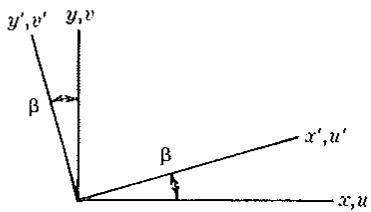
Figure 7.3-1. The two-dimensional case. Coordinate systems $xy$ and $x'y'$ , with table of direction cosines between axes. Thus $[T_{\epsilon}]^{-T}$ is obtained from $[T_{\epsilon}]$ by shifting factors of 2 in $[T_{\epsilon}]$ symmetrically about the diagonal. Material Properties. A single stress-strain relation can be written as $\{\sigma\} = [\mathbf{E}]\{\epsilon\}$ in the xyz coordinate system or as $\{\sigma'\} = [\mathbf{E}']\{\epsilon'\}$ in the $x'y'z'$ coordinate system. Imagine that $[\mathbf{E}']$ is known and $[\mathbf{E}]$ is desired. By substitution from Eqs. 7.3-4, 7.3-7, and the relation $\{\sigma'\} = [\mathbf{E}']\{\epsilon'\}$ , $$ \{\boldsymbol {\sigma} \} = [ \mathbf {T} _ {\epsilon} ] ^ {T} \{\boldsymbol {\sigma} ^ {\prime} \} = [ \mathbf {T} _ {\epsilon} ] ^ {T} [ \mathbf {E} ^ {\prime} ] \{\boldsymbol {\epsilon} ^ {\prime} \} = [ \mathbf {T} _ {\epsilon} ] ^ {T} [ \mathbf {E} ^ {\prime} ] [ \mathbf {T} _ {\epsilon} ] \{\boldsymbol {\epsilon} \} \tag {7.3-9} $$ from which $$ [ \mathbf {E} ] = [ \mathbf {T} _ {\epsilon} ] ^ {T} [ \mathbf {E} ^ {\prime} ] [ \mathbf {T} _ {\epsilon} ] \tag {7.3-10} $$ This transformation concerns conditions at a point. Therefore, it is not necessary that xyz and $x'y'z'$ be Cartesian systems. For example, one coordinate system might be Cartesian and the other cylindrical. Plane Problems. A two-dimensional problem is a special case in which $n_3 = 1$ and $\ell_3 = m_3 = n_1 = n_2 = 0$ (see Fig. 7.3-1). In the $xy$ plane, $\{\epsilon\} = \left\lfloor \epsilon_x \quad \epsilon_y \quad \gamma_{xy} \right\rfloor^T$ , $\{\sigma\} = \left\lfloor \sigma_x \quad \sigma_y \quad \tau_{xy} \right\rfloor^T$ , [E] is 3 by 3, and $$ \left[ \mathbf {T} _ {\epsilon} \right] = \left[ \begin{array}{c c c} c ^ {2} & s ^ {2} & c s \\ s ^ {2} & c ^ {2} & - c s \\ - 2 c s & 2 c s & c ^ {2} - s ^ {2} \end{array} \right] \quad \text { and } \quad \left[ \mathbf {T} _ {\epsilon} \right] ^ {- T} = \left[ \begin{array}{c c c} c ^ {2} & s ^ {2} & 2 c s \\ s ^ {2} & c ^ {2} & - 2 c s \\ - c s & c s & c ^ {2} - s ^ {2} \end{array} \right] \tag {7.3-11} $$ where $c = \cos \beta$ and $s = \sin \beta$ . Hence, one can recognize Eqs. 7.3-7 as the familiar Mohr's circle relations used in elementary mechanics of materials. # 7.4 TRANSFORMATION OF STIFFNESS MATRICES In two coordinate systems such as xyz and $x'y'z'$ , the element stiffness relation can be written as $$ [ \mathbf {k} ] \{\mathbf {d} \} = \{\mathbf {r} \} \quad \text { or as } \quad [ \mathbf {k} ^ {\prime} ] \{\mathbf {d} ^ {\prime} \} = \{\mathbf {r} ^ {\prime} \} \tag {7.4-1} $$ The stiffness matrix of a given element can be expressed as either [k] or [k']. The two matrices differ because they operate on different nodal d.o.f.—namely, {d} and {d'. We imagine here that [k'] is known and [k] is desired. The necessary transformation is now derived. A review of the argument associated with Eqs. 7.2-5 and 7.2-6 shows that no special form need be assumed for the matrix that relates $\{\mathbf{d}'\}$ and $\{\mathbf{d}\}$ . It is required only that the relation be known. We will call the relational matrix [T]. The argument of Eqs. 7.2-5 and 7.2-6 is that $$ \text { if } \quad \{\mathbf {d} ^ {\prime} \} = [ \mathbf {T} ] \{\mathbf {d} \} \quad \text { then } \quad \{\mathbf {r} \} = [ \mathbf {T} ] ^ {T} \{\mathbf {r} ^ {\prime} \} \tag {7.4-2} $$ Examples will follow. For now we remark only that $\{d\}$ and $\{d'\}$ need not be the same size and need not even contain the same kind of d.o.f. Hence, the stiffness transformation is easy to derive. By substitution of Eqs. 7.4-2 into Eq. 7.4-1, $$ [ \mathbf {k} ] \{\mathbf {d} \} = \{\mathbf {r} \} = [ \mathbf {T} ] ^ {T} \{\mathbf {r} ^ {\prime} \} = [ \mathbf {T} ] ^ {T} [ \mathbf {k} ^ {\prime} ] \{\mathbf {d} ^ {\prime} \} = [ \mathbf {T} ] ^ {T} [ \mathbf {k} ^ {\prime} ] [ \mathbf {T} ] \{\mathbf {d} \} \tag {7.4-3} $$ from which $$ [ \mathbf {k} ] = [ \mathbf {T} ] ^ {T} [ \mathbf {k} ^ {\prime} ] [ \mathbf {T} ] \tag {7.4-4} $$ Equation 7.4-4 does not change the orientation of the element in fixed global coordinates or alter element properties; rather, this transformation alters the formal expression of element properties to agree with a change of d.o.f. from $\{\mathbf{d}'\}$ to $\{\mathbf{d}\}$ . For future reference, we note that mass and damping matrices used in dynamics transform in the same way. That is, $[m] = [T]^{T}[m'][T]$ and $[c] = [T]^{T}[c'][T]$ . 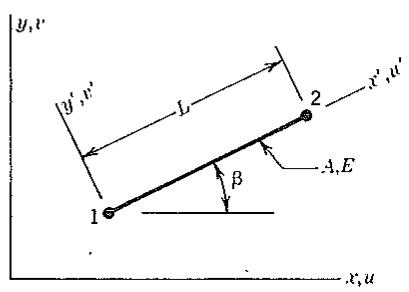# 7.5 EXAMPLES: TRANSFORMATION OF STIFFNESS MATRICES Plane Truss Element. Imagine that the stiffness matrix of the bar in Fig. 7.5-1a in local coordinates $x'y'$ is called $[k']$ and is known. From it, $[k]$ is to be determined, where $[k]$ is the stiffness matrix of the bar referred to global coordinates xy. Thus $[k']$ and $[k]$ describe the same bar but use different d.o.f. to do so. We have $$ \left[ \mathbf {k} ^ {\prime} \right] = \frac {A E}{L} \left[ \begin{array}{c c c c} 1 & 0 & - 1 & 0 \\ 0 & 0 & 0 & 0 \\ - 1 & 0 & 1 & 0 \\ 0 & 0 & 0 & 0 \end{array} \right] \quad \text { and } \quad \left\{ \begin{array}{l} u _ {1} ^ {\prime} \\ v _ {1} ^ {\prime} \\ u _ {2} ^ {\prime} \\ v _ {2} ^ {\prime} \end{array} \right\} = \left[ \begin{array}{c c c c} c & s & 0 & 0 \\ - s & c & 0 & 0 \\ 0 & 0 & c & s \\ 0 & 0 & - s & c \end{array} \right] \left\{ \begin{array}{l} u _ {1} \\ v _ {1} \\ u _ {2} \\ v _ {2} \end{array} \right\} \tag {7.5-1} $$ where $c = \cos \beta$ and $s = \sin \beta$ . The square matrix of sines and cosines is [T]. It is built from matrices [A] of Eq. 7.2-1, specialized to two dimensions (Fig. 7.3-1). We find that [k] = [T] $^{7}$ [k′][T] is the stiffness matrix given by Eq. 2.4-3, as expected. However, the foregoing procedure involves unnecessary effort. Terms in rows 

text_image

y,v y',v' L 2 x',u' β A,E 1 x,u

(n) 

text_image

y,v y',v' L x',u' 1 A,E z',w' z,w r,u

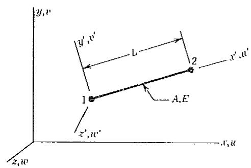
(b) Figure 7.5-1. A uniform two-force (bar or truss) element in local and global reference frames. (a) Two-dimensional case. (b) Three-dimensional case. 2 and 4 of [T], which pertain to $v_1'$ and $v_2'$ , are always multiplied by zero. This is physically reasonable, as axis $x'$ completely defines the orientation of the element. Rather than use Eqs. 7.5-1, it is more efficient to use for [k'] the 2 by 2 matrix in Eq. 2.4-5. Thus $$ [ \mathbf {k} ^ {\prime} ] = \frac {A E}{L} \left[ \begin{array}{c c} 1 & - 1 \\ - 1 & 1 \end{array} \right] \quad \text { and } \quad \left\{ \begin{array}{l} u _ {1} ^ {\prime} \\ u _ {2} ^ {\prime} \end{array} \right\} = [ \mathbf {T} ] \left\{ \begin{array}{l} u _ {1} \\ v _ {1} \\ u _ {2} \\ v _ {2} \end{array} \right\} \tag {7.5-2} $$ where, with $c = \cos \beta$ and $s = \sin \beta$ , $$ [ \mathbf {T} ] _ {2 \times 4} = \left[ \begin{array}{l l l l} c & s & 0 & 0 \\ 0 & 0 & c & s \end{array} \right] \tag {7.5-3} $$ With $[k']$ and $[T]$ thus defined, the operation $[k] = [T]^{T}[k'][T]$ again produces the expected 4 by 4 matrix of Eq. 2.4-3. Space Truss Element. With $[k']$ again defined as in Eq. 7.5-2, we wish to obtain from it the 6 by 6 matrix $[k]$ for the element in Fig. 7.5-1b, which operates on nodal displacements parallel to x, y, and z axes. Vectors of local and global d.o.f. for this element are $$ \{\mathbf {d} ^ {\prime} \} = \left[ \begin{array}{l l} u _ {1} ^ {\prime} & u _ {2} ^ {\prime} \end{array} \right] ^ {T} \quad \text { and } \quad \{\mathbf {d} \} = \left[ \begin{array}{l l l l l l} u _ {1} & v _ {1} & w _ {1} & u _ {2} & v _ {2} & w _ {2} \end{array} \right] ^ {T} \tag {7.5-4} $$ The transformation is $\{\mathbf{d}'\} = [\mathbf{T}]\{\mathbf{d}\}$ , where $$ \left[ \begin{array}{l} \mathbf {T} \\ 2 \times 6 \end{array} \right] = \left[ \begin{array}{c c c c c c} \ell_ {1} & m _ {1} & n _ {1} & 0 & 0 & 0 \\ 0 & 0 & 0 & \ell_ {1} & m _ {1} & n _ {1} \end{array} \right] \tag {7.5-5} $$ and $\ell_1, m_1$ , and $n_1$ are direction cosines of axis $x'$ . The desired result is $[\mathbf{k}] = [\mathbf{T}]^T[\mathbf{k}'][\mathbf{T}]$ . Plane Frame Element. This element is a plane beam but with axial deformation permitted. We first write the stiffness matrix $[k']$ in local coordinates $x'y'$ , Fig. 

text_image

y' L v2' u2' x' r1' A,E,I θ2' u1' θ1'

$$ Z = A E / L \quad K = 1 2 E I / L ^ {3} $$ $$ A = 4 E I / L \quad M = 6 E I / L ^ {2} $$ $$ B = 2 E I / L $$ 

text_image

y L v2 u2 v1 A,E,I θ2 β u1 x θ1 c = cosβ s = sinβ

$$ F = Z c ^ {2} + K s ^ {2} \quad H = - M s $$ $$ G = (Z - K) c s \quad Q = M c $$ $$ P = Z s ^ {2} + K c ^ {2} $$ $$ \left[ \begin{array}{c c c c c c} Z & 0 & 0 & - Z & 0 & 0 \\ 0 & K & M & 0 & - K & M \\ 0 & M & A & 0 & - M & B \\ - Z & 0 & 0 & Z & 0 & 0 \\ 0 & - K & - M & 0 & K & - M \\ 0 & M & B & 0 & - M & A \end{array} \right] $$ $[\mathbf{k}^{\prime}]$ (for primed d.o.f.) (a) $$ \left[ \begin{array}{c c c c c c} F & G & H & - F & - G & H \\ G & P & Q & - G & - P & Q \\ H & Q & A & - H & - Q & B \\ - F & - G & - H & F & G & - H \\ - G & - P & - Q & G & P & - Q \\ H & Q & B & - H & - Q & A \end{array} \right] $$ [k] (for unprimed d.o.f.) (b) 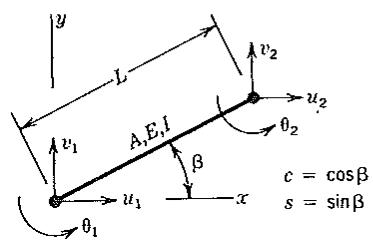Figure 7.5-2. The stiffness matrix of a uniform plane frame element. 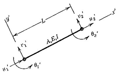7.5-2a. The element can both stretch and bend in the $xy$ (or the $x'y'$ ) plane. Element stiffness matrix $[\mathbf{k}']$ operates on the d.o.f. $$ \left\{\mathbf {d} ^ {\prime} \right\} = \left\lfloor u _ {1} ^ {\prime} v _ {1} ^ {\prime} \theta_ {1} ^ {\prime} u _ {2} ^ {\prime} v _ {2} ^ {\prime} \theta_ {2} ^ {\prime} \right] ^ {T} \tag {7.5-6} $$ D.o.f. $u_{1}^{\prime}$ and $u_{2}^{\prime}$ are associated with axial stiffness AE/L. The remaining d.o.f. are associated with bending. Axial and bending effects do not interact (unless a large axial load produces “beam–column” action). We therefore create the 6 by 6 matrix $[k^{\prime}]$ of the frame element by taking terms from the beam element matrix (Eq. 4.2-5) and the truss element matrix (Eq. 7.5-1). The resulting $[k^{\prime}]$ appears in Fig. 7.5-2a. To generate [k] in global coordinates $xy$ we apply Eq. 7.4-4. The transformation matrix is $$ \left[ \begin{array}{l} \mathbf {T} \\ 6 \times 6 \end{array} \right] = \left[ \begin{array}{l l} \mathbf {T} _ {n} & \mathbf {0} \\ \mathbf {0} & \mathbf {T} _ {n} \end{array} \right], \quad \text { where } \quad \left[ \begin{array}{l} \mathbf {T} _ {n} \end{array} \right] = \left[ \begin{array}{l l l} \cos \beta & \sin \beta & 0 \\ - \sin \beta & \cos \beta & 0 \\ 0 & 0 & 1 \end{array} \right] \tag {7.5-7} $$ The “1” appears in $[T_{n}]$ because the rotation vectors do not change in direction: $\theta_{1}^{\prime} = \theta_{1}$ and $\theta_{2}^{\prime} = \theta_{2}$ . The [k] that results from transformation, and the d.o.f. on which it operates, are shown in Fig. 7.5-2b. # 7.6 INCLINED SUPPORT Consider a structure that has translational nodal d.o.f. directed along the coordinate axes xyz. It may happen that a certain node is allowed to move only in a 

text_image

y,v s,V 4 2 3 1 x,u β r,U

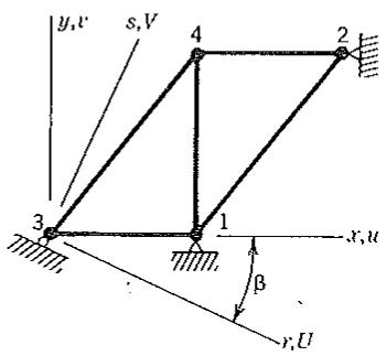
Figure 7.6-1. A plane truss or plane frame in which node 3 is allowed to move in only the r direction. plane that is not parallel to a coordinate plane. In other words, displacement is prohibited in a direction that is not parallel to x, y, or z axes. A way to treat this boundary condition is now illustrated by using a plane structure. In Fig. 7.6-1, the inclined support requires that $v_{3} = -u_{3} \tan \beta$ (or, in terms of other d.o.f., it requires that $V_{3} = 0$ while $U_{3}$ is unrestrained). It is easier to deal with the constraint $V_{3} = 0$ than with the constraint $v_{3} = -u_{3} \tan \beta$ . The procedure described in the following replaces $u_{3}$ and $v_{3}$ by $U_{3}$ and $V_{3}$ without changing other d.o.f. of the structure. One then uses a standard method to set $V_{3} = 0$ (see Section 2.10). $U_{3}$ remains active and is computed as part of the solution vector $\{D\}$ in the usual way. Before any support conditions are imposed in Fig. 7.6-1, the structure stiffness equations $[K]\{D\} = \{R\}$ , partitioned by node, are $$ \left[ \begin{array}{c c c c} \mathbf {K} _ {1 1} & \mathbf {K} _ {1 2} & \mathbf {K} _ {1 3} & \mathbf {K} _ {1 4} \\ \mathbf {K} _ {2 1} & \mathbf {K} _ {2 2} & \mathbf {0} & \mathbf {K} _ {2 4} \\ \mathbf {K} _ {3 1} & \mathbf {0} & \mathbf {K} _ {3 3} & \mathbf {K} _ {3 4} \\ \mathbf {K} _ {4 1} & \mathbf {K} _ {4 2} & \mathbf {K} _ {4 3} & \mathbf {K} _ {4 4} \end{array} \right] \left\{ \begin{array}{l} \mathbf {D} _ {1} \\ \mathbf {D} _ {2} \\ \mathbf {D} _ {3} \\ \mathbf {D} _ {4} \end{array} \right\} = \left\{ \begin{array}{l} \mathbf {R} _ {1} \\ \mathbf {R} _ {2} \\ \mathbf {R} _ {3} \\ \mathbf {R} _ {4} \end{array} \right\} \tag {7.6-1} $$ where, depending on whether the structure is a plane truss or a plane frame, $$ \{\mathbf {D} _ {i} \} = \left[ \begin{array}{l l} u _ {i} & v _ {i} \end{array} \right] ^ {T} \quad \text { or } \quad \{\mathbf {D} _ {i} \} = \left[ \begin{array}{l l l} u _ {i} & v _ {i} & \theta_ {i} \end{array} \right] ^ {T} \tag {7.6-2} $$ To replace $u_{3}$ and $v_{3}$ by $U_{3}$ and $V_{3}$ , we write the transformation relation $$ \left\{ \begin{array}{l} u _ {3} \\ v _ {3} \end{array} \right\} = [ \mathbf {T} _ {3} ] \left\{ \begin{array}{l} U _ {3} \\ V _ {3} \end{array} \right\}. \quad \text { or } \quad \left\{ \begin{array}{l} u _ {3} \\ v _ {3} \\ \theta_ {3} \end{array} \right\} = [ \mathbf {T} _ {3} ] \left\{ \begin{array}{l} U _ {3} \\ V _ {3} \\ \theta_ {3} \end{array} \right\} \tag {7.6-3} $$ where, with $c = \cos \beta$ and $s = \sin \beta$ , $$ \left[ \mathrm{T} _ {3} \right] = \left[ \begin{array}{c c} c & s \\ - s & c \end{array} \right] \quad \text { or } \quad \left[ \mathrm{T} _ {3} \right] = \left[ \begin{array}{c c c} c & s & 0 \\ - s & c & 0 \\ 0 & 0 & 1 \end{array} \right] \tag {7.6-4} $$ for plane truss and plane frame, respectively. The transformation matrix [T] for the entire structure is a unit matrix except for $[T_{3}]$ on the diagonal. With [I] a 2 by 2 or a 3 by 3 unit matrix, [T] is $$ [ \mathbf {T} ] = \left[ \begin{array}{l l l l} \mathbf {I} & \mathbf {I} & \mathbf {T} _ {3} & \mathbf {I} \end{array} \right] \tag {7.6-5} $$ After Eq. 7.6-1 is transformed, $\lfloor U_3 \quad V_3 \rfloor^T$ or $\lfloor U_3 \quad V_3 \quad \theta_3 \rfloor^T$ replaces $\{\mathbf{D}_3\}$ , $[\mathbf{T}_3]^T\{\mathbf{R}_3\}$ replaces $\{\mathbf{R}_3\}$ , and the structure stiffness matrix becomes $$ [ \mathbf {T} ] ^ {T} [ \mathbf {K} ] [ \mathbf {T} ] = \left[ \begin{array}{c c c c} \mathbf {K} _ {1 1} & \mathbf {K} _ {1 2} & \mathbf {K} _ {1 3} \mathbf {T} _ {3} & \mathbf {K} _ {1 4} \\ \mathbf {K} _ {2 1} & \mathbf {K} _ {2 2} & \mathbf {0} & \mathbf {K} _ {2 4} \\ \mathbf {T} _ {3} ^ {T} \mathbf {K} _ {3 1} & \mathbf {0} & \mathbf {T} _ {3} ^ {T} \mathbf {K} _ {3 3} \mathbf {T} _ {3} & \mathbf {T} _ {3} ^ {T} \mathbf {K} _ {3 4} \\ \mathbf {K} _ {4 1} & \mathbf {K} _ {4 2} & \mathbf {K} _ {4 3} \mathbf {T} _ {3} & \mathbf {K} _ {4 4} \end{array} \right] \tag {7.6-6} $$ Transformed arrays [K] and {R} can be transformed again if there is another skew support. Conceivably, all nodes of the truss or frame could be skew and all translational d.o.f. in {D} could have different directions. If n successive transformations are used so that $\{D'\} = [T_{1}]\{D\}$ , $\{D''\} = [T_{2}]\{D'\}$ , and so on, original d.o.f. $\{D^{n}\}$ are related to final d.o.f. {D} by the equation $$ \{\mathbf {D} ^ {n} \} = [ \mathbf {T} _ {n} ] [ \mathbf {T} _ {n - 1} ] \cdot \cdot \cdot [ \mathbf {T} _ {1} ] \{\mathbf {D} \}. \tag {7.6-7} $$ In the preceding explanation, transformation is done at the structure level. This approach requires that we construct and use [T] in a manner consistent with whatever compact storage format has been adopted for the structure stiffness matrix. It also requires that a d.o.f. to be suppressed (e.g., $V_{3}$ in Fig. 7.6-1) remain present until transformation is complete. If, instead, the separate element matrices are transformed before assembly, the scheme of Figs. 2.10-4 and 2.10-5 can be used to exclude from $\{D\}$ the d.o.f. to be suppressed. The required transformation matrix for a plane frame element, with all six of its d.o.f. included, is $$ [ \mathbf {T} ] _ {6 \times 6} = \left[ \begin{array}{l l} \mathbf {T} _ {3} & \mathbf {0} \\ \mathbf {0} & \mathbf {I} \end{array} \right] \quad \text { or } \quad [ \mathbf {T} ] _ {6 \times 6} = \left[ \begin{array}{l l} \mathbf {I} & \mathbf {0} \\ \mathbf {0} & \mathbf {T} _ {3} \end{array} \right] \tag {7.6-8} $$ depending on which node of the element coincides with the affected node of the frame. This transformation must be applied to every element that is attached to the affected node (node 3 in Fig. 7.6-1). 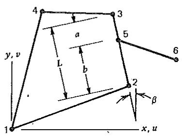# 7.7 JOINING DISSIMILAR ELEMENTS TO ONE ANOTHER An element match termed “dissimilar” is depicted in Fig. 7.7-1a. The left end of a plane frame element is to be attached at an arbitrary location along an edge of a plane four-node quadrilateral element. Node 5 of the frame element does not coincide with a node of the quadrilateral. Moreover, rotational d.o.f. appear at nodes 5 and 6, but nodes 1 through 4 have only translational d.o.f. A method of connecting these two elements is now described. The frame element stiffness relation is $[\mathbf{k}']\{\mathbf{d}'\} = \{\mathbf{r}'\}$ , where $$ \{\mathbf {d} ^ {\prime} \} = \left\lfloor u _ {5} v _ {5} \theta_ {5} u _ {6} v _ {6} \theta_ {6} \right\rfloor^ {T} \tag {7.7-1} $$ We seek modified matrices $[\mathbf{k}]$ and $\{\mathbf{r}\}$ for the frame element, where $$ [ \mathbf {k} ] = [ \mathbf {T} ] ^ {T} [ \mathbf {k} ^ {\prime} ] [ \mathbf {T} ] \quad \text { and } \quad \{\mathbf {r} \} = [ \mathbf {T} ] ^ {T} \{\mathbf {r} ^ {\prime} \} \tag {7.7-2} $$ 

text_image

4 3 a L b 2 6 y, v 1 x, u β

[a] 

text_image

L₂ c 4 y, v 3 a 6 b L₁ d 5 1 2 x, u

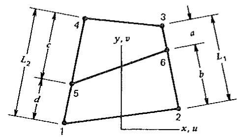
{b} Figure 7.7-1. (a) A standard plane frame element connected to a four-node plane element. (b) A two-force (bar) element connected to a four-node plane element. New d.o.f. of the frame element are to be $$ \{\mathbf {d} \} = \left[ \begin{array}{l l l l l l l} u _ {2} & v _ {2} & u _ {3} & v _ {3} & u _ {6} & v _ {6} & \theta_ {6} \end{array} \right] ^ {T} \tag {7.7-3} $$ In the expression $\{\mathbf{d}'\} = [\mathbf{T}]\{\mathbf{d}\}$ , transformation matrix [T] is written by saying that translational motion of node 5 is linearly interpolated along edge 2-3 from translational d.o.f. at nodes 2 and 3, and that rotation $\theta_{5}$ is the same as the rotation of edge 2-3. Thus, with $c = \cos \beta$ and $s = \sin \beta$ , $$ [ \mathbf {T} ] _ {6 \times 7} = \left[ \begin{array}{l l} \mathbf {T} _ {3} & \mathbf {0} \\ \mathbf {0} & \mathbf {I} \end{array} \right], \quad \text { where } \quad [ \mathbf {T} _ {3} ] = \frac {1}{L} \left[ \begin{array}{c c c c} a & 0 & b & 0 \\ 0 & a & 0 & b \\ c & s & - c & - s \end{array} \right] \tag {7.7-4} $$ and $[I]=\left[\begin{matrix}1&1&1\end{matrix}\right]$ . We see that $[k]$ is a 7 by 7 matrix. Quadrilateral and frame elements can now be assembled to one another or assembled into the rest of the structure. Node 5 and its d.o.f. do not appear in the assembled structure. Node 5 may be called a “slave” node because its d.o.f. are completely determined by d.o.f. of “master” nodes 2 and 3. As a second example, consider the problem of Fig. 7.7-1b. A two-force member, perhaps a reinforcing bar in concrete, is to be connected to points arbitrarily located along edges of a plane four-node element. Matrices $\{r'\}$ and $[k']$ of the bar are associated with d.o.f. $u_{5}$ , $v_{5}$ , $u_{6}$ , and $v_{6}$ . By transformation, $\{r'\}$ and $[k']$ are to be converted to $\{r\}$ and $[k]$ , which are associated with d.o.f. $u_{i}$ and $v_{i}$ of the four corner nodes of the quadrilateral, i = 1, 2, 3, 4. Thus $$ \left\{\mathbf {r} ^ {\prime} \right\} _ {4 \times 1} ^ {\cdot} \text { becomes } \left\{\mathbf {r} \right\} _ {8 \times 1} \text { and } \left[ \mathbf {k} ^ {\prime} \right] _ {4 \times 4.} \text { becomes } \left[ \mathbf {k} \right] _ {8 \times 8} \tag {7.7-5} $$ The displacement transformation for d.o.f. $\{d'\}$ of the bar is $\{d'\} = [T]\{d\}$ , and the required transformation matrix [T] is 4 by 8. With displacements linearly interpolated along edges of the quadrilateral, [T] contains terms like those in the first two rows of $[T_{3}]$ in Eq. 7.7-4. After transformation, $\{r\}$ and $[k]$ can be directly added to the corresponding arrays of the quadrilateral or assembled into the structure. Nodes 5 and 6 and their d.o.f. are then not explicitly present. One can say that d.o.f. of the frame and bar elements in Fig. 7.7-1 are constrained to follow d.o.f. of the quadrilateral. $^{2}$ # 7.8 RIGID LINKS. RIGID ELEMENTS Rigid members impose relationships among d.o.f. This circumstance is sometimes called a multipoint constraint. $^{3}$ In the present section we consider rigid members as an application of coordinate transformation. 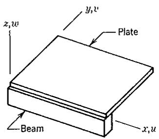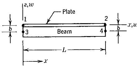Rigid Links. Imagine that a plate is to be reinforced by a beam (Fig. 7.8-1). Nodes of the beam do not coincide with nodes of the plate. (If nodes were coincident, the beam-plate connection would be easy; one would simply assemble elements in the usual way.) Even with an offset beam, it is still possible to connect beam and plate in such a way that d.o.f. of only the plate appear in the assembled structure. The procedure for doing so is now described. The procedure invokes a transformation that makes beam d.o.f. at nodes 3 and 4 “slave” to “master” d.o.f. at nodes 1 and 2 in the plate. This is accomplished by adding imaginary, weightless, rigid links—one between nodes 1 and 3 and another between nodes 2 and 4. We assume that the beam has bending stiffness (associated with d.o.f. $w_{3}$ , $\theta_{3}$ , $w_{4}$ , and $\theta_{4}$ ) and axial stiffness (associated with d.o.f. $u_{3}$ and $u_{4}$ ). These six d.o.f. must be incorporated in the transformation relation. At the left end, the transformation is $$ \left\{ \begin{array}{l} u _ {3} \\ w _ {3} \\ \theta_ {3} \end{array} \right\} = [ \mathbf {T} _ {\ell} ] \left\{ \begin{array}{l} u _ {1} \\ w _ {1} \\ \theta_ {1} \end{array} \right\}, \quad \text { where } \quad [ \mathbf {T} _ {\ell} ] = \left[ \begin{array}{l l l} 1 & 0 & b \\ 0 & 1 & 0 \\ 0 & 0 & 1 \end{array} \right] \tag {7.8-1} $$ A similar transformation is written at the right end by replacing subscripts 1 by 2 and 3 by 4. We see that d.o.f. $u_{3}$ and $u_{4}$ are activated by $\theta_{1}$ and $\theta_{2}$ . Thus, because of the rigid links, axial stiffness of the beam is seen as bending stiffness by the plate d.o.f. Let $\{\mathbf{r}'\}$ and $[\mathbf{k}']$ be beam element matrices associated with d.o.f. at nodes 3 and 4 (see Fig. 7.5-2a for $[\mathbf{k}']$ ). Transformed arrays $\{\mathbf{r}\}$ and $[\mathbf{k}]$ , associated with d.o.f. at plate nodes 1 and 2, are $$ \begin{array}{l} \{\mathbf {r} \} = [ \mathbf {T} ] ^ {T} \{\mathbf {r} ^ {\prime} \} \\ [ \mathbf {k} ] = [ \mathbf {T} ] ^ {T} [ \mathbf {k} ^ {\prime} ] [ \mathbf {T} ] \end{array} \quad \text { where } \quad \begin{array}{l} [ \mathbf {T} ] = \left[ \begin{array}{c c} \mathbf {T} _ {\ell} & \mathbf {0} \\ \mathbf {0} & \mathbf {T} _ {\ell} \end{array} \right] \\ 6 \times 6 \end{array} \tag {7.8-2} $$ 

text_image

z,w y,v Plate Beam x,u

(a) 

text_image

z,w Plate 1 2 x,u 3 Beam 4 b b L x

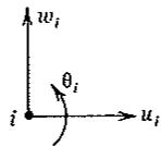
(b)  (c) Figure 7.8-1. (a) A reinforcing beam joined to one edge of a plate element. (b) Side view. (c) Typical node i (i = 1, 2, 3, 4), showing d.o.f. considered in the coordinate transformation. $^{3}$ Constraints are discussed in detail in Chapter 9.