```lua C--- Do condensation operations on lower triangle of SE. DO 30 K=1, NUM LL = NSIZE - K KK = LL + 1 DO 20 L=1, LL DUM = SE(KK, L)/SE(KK, KK) DO 10 M=1, L 10 SE(L, M) = SE(L, M) - SE(KK, M) * DUM RE(L) = RE(L) - RE(KK) * DUM 20 CONTINUE 30 CONTINUE C--- Fill in the upper triangle of SE by symmetry. DO 40 K=1, LL DO 40 L=1, K 40 SE(L, K) = SE(K, L) ``` Figure 8.2-1. A Fortran condensation algorithm that accepts a symmetric matrix, stored in full rather than banded format, does Gauss elimination from the bottom with diagonal pivots and yields the condensed [k] and {r} of Eq. 8.1-3. # 8.2 CONDENSATION AND RECOVERY ALGORITHMS Our algorithm is a straightforward coding of Gauss elimination to produce the condensed arrays [k] and {r} of Eqs. 8.1-3 from the uncondensed arrays of Eq. 8.1-1. Let there be NSIZE d.o.f. in the uncondensed system, and let it be required to condense the last NUM of these d.o.f. In Fig. 8.2-1 condensation is done in place, so that after completion of the condensation algorithm, the condensed [k] resides in the upper left NSIZE-NUM rows and columns of array SE, and the condensed {r} resides in the upper NSIZE-NUM rows of array RE. After structural equations have been solved, d.o.f. $\{d_{r}\}$ reside in the structure solution vector $\{D\}$ . It remains to recover $\{d_{c}\}$ in Eq. 8.1-2. This can be done by back-substitution, thus completing the Gauss elimination solution that was begun by condensation. Figure 8.2-2 gives the Fortran coding. In Fig. 8.2-2, arrays SM and RM contain the last NUM rows of arrays SE and RE exactly as they stand after completion of the condensation routine. In Fig. 8.2-1 these rows follow the condensed matrices, and are numbered NUM+1 through NSIZE. In Fig. 8.2-2 these rows are duplicated in arrays SM and RM, where they occupy rows 1 through NUM. In Fig. 8.2-2 the first NSIZE-NUM rows of array DE contain the known d.o.f. $\{d_{r}\}$ . Internal d.o.f. $\{d_{c}\}$ are computed and stored in the last NUM rows of array DE. In the foregoing algorithms, mass storage would probably be used to store the last NUM rows of arrays SE and RE from Fig. 8.2-1. Node point coordinates, and $\{\epsilon_{0}\}$ and $\{\sigma_{0}\}$ , would also be stored. After $\{D\}$ is known, these data would be recalled and Fig. 8.2-2 used to compute $\{d_{c}\}$ . At each point where stresses are needed, [B] can be reconstructed from the node point coordinates. Finally, strains are $\{\epsilon\} = [B]\left[d_{r} \cdot d_{c}\right]^{T} - \{\epsilon_{0}\}$ and stresses are $\{\sigma\} = [E]\{\epsilon\} + \{\sigma_{0}\}$ . ```txt DO 60 J=1, NUM JJ = NSIZE - NUM + J DUM = 0. K = JJ - 1 DO 50 L=1, K 50 DUM = DUM + SM(J, L)*DE(L) 60 DE(JJ) = (RM(J) - DUM)/SM(J, JJ) ``` Figure 8.2-2. Recovery of previously condensed d.o.f. $\{d_{c}\}$ when $\{d_{r}\}$ and $\{r_{c}\}$ are known. Alternative Method. In an alternative method [8.1], explicit recovery of $\{d_{c}\}$ is avoided. Instead, as part of the process of generating the element stiffness matrix, an element stress matrix [S] and stress vector $\{\rho\}$ are also generated. After element d.o.f. $\{d_{r}\}$ are known, element stresses $\{\sigma\}$ are computed by the equation $$ \{\pmb {\sigma} \} = [ \mathbf {S} ] \{\mathbf {d} _ {r} \} + \{\pmb {\rho} \} \tag {8.2-1} $$ in which previously condensed d.o.f. $\{\mathbf{d}_c\}$ do not appear. The most significant differences between the two methods are as follows. The first method, Figs. 8.2-1 and 8.2-2, explicitly recovers $\{d_{c}\}$ and reconstructs a (somewhat sparse) matrix [B] at each stress point. The alternative method generates, condenses, and stores an array [S] that is smaller than [B] but not sparse. Both methods yield the same stresses. The relative cost of the two methods depends on billing charges for computing and for mass storage, the size of $\{d_{r}\}$ in relation to $\{d_{c}\}$ , the number of load conditions, the number of stress points, and other less important factors. The method of Figs. 8.2-1 and 8.2-2 tends to be cheaper if $\{d_{c}\}$ is small in relation to $\{d_{r}\}$ , if the number of load cases is small, or if the number of stress points is large. Further comparison appears in [8.2]. # 8.3 PARASITIC SHEAR. 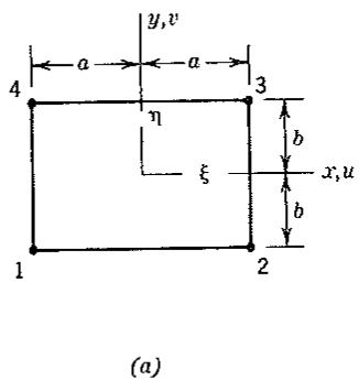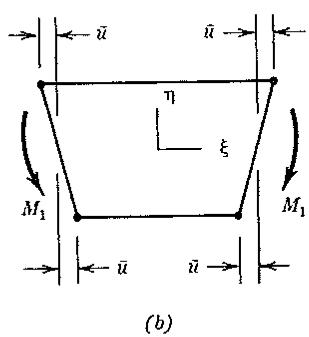INCOMPATIBLE ELEMENTS Parasitic Shear. Bilinear elements, discussed in Section 6.3, are attractive because they are simple and have only corner nodes. Unfortunately, they are too stiff in bending, whether the element is a rectangle or an arbitrary quadrilateral. We illustrate the point with reference to the rectangular element in Fig. 8.3-1. Here $\xi$ and $\eta$ are dimensionless Cartesian coordinates, $\xi = x/a$ and $\eta = y/b$ . Let bending moment $M_{1}$ be applied, so that nodal displacements $\overline{u}$ arise in response, as shown in Fig. 8.3-1b. According to Eqs. 6.3-2 and 6.3-16, the element deformation field is $$ u = \xi \eta \overline {{{u}}} \qquad \text { and } \qquad v = 0 \tag {8.3-1} $$ Thus top and bottom edges $\eta = \pm 1$ remain straight, and strains in the element are 

text_image

y,v a a 4 3 η ξ b x,u b 1 2 (a)


text_image

ū ū η ξ M₁ M₁ ū ū (b)


text_image

M₂ η ξ M₂ (c)

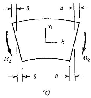
Figure 8.3-1. (a) A rectangular bilinear element. (b) The bilinear element deformed by bending moment $M_{1}$ . (c) Correct deformed geometry for pure bending under bending moment $M_{2}$ . $$ \epsilon_ {x} = \eta \frac {\overline {{{u}}}}{a} \quad \epsilon_ {y} = 0 \quad \gamma_ {x y} = \xi \frac {\overline {{{u}}}}{b} \tag {8.3-2} $$ The correct shape under pure bending, Fig. 8.3-1c, is $$ u = \xi \eta \overline {{u}} \quad \text { and } \quad v = (1 - \xi^ {2}) \frac {a \overline {{u}}}{2 b} + (1 - \eta^ {2}) \nu \frac {b \overline {{u}}}{2 a} \tag {8.3-3} $$ where $\nu$ is Poisson's ratio. From Eqs. 8.3-3, the correct strains under pure bending are $$ \epsilon_ {x} = \eta \frac {\overline {{{u}}}}{a} \quad \epsilon_ {y} = - \nu \eta \frac {\overline {{{u}}}}{a} \quad \gamma_ {x y} = 0 \tag {8.3-4} $$ Upon comparing Eqs. 8.3-2 and 8.3-4, we see that if bending displacements $\overline{u}$ are imposed, the correct behavior gives rise to storage of strain energy caused by normal strains alone, but the bilinear element stores strain energy caused by normal strain $\epsilon_{x}$ and a spurious shear strain $\gamma_{xy}$ . Thus, for the same deformation, $M_{1} > M_{2}$ in Fig. 8.3-1. Specifically, by computing the ratio of strain energies in the two cases, we obtain $$ \frac {M _ {1}}{M _ {2}} = \frac {1}{1 + \nu} \left[ \frac {1}{1 - \nu} + \frac {1}{2} \left(\frac {a}{b}\right) ^ {2} \right] \tag {8.3-5} $$ The unwanted shear strain that produces $M_{1} > M_{2}$ is called parasitic shear. Equation 8.3-5 shows that its effect is disastrous if a/b is large; that is, for large a/b the mesh “locks.” Locking is discussed in more detail in Section 9.4. Incompatible Elements. Upon comparing Eqs. 8.3-1 and 8.3-3, we see that the bilinear element errs by omitting from v the displacement modes associated with $(1 - \xi^{2})$ and $(1 - \eta^{2})$ . In the bending mode where $v = \overline{v}\xi\eta$ , similar modes are omitted from u. The eight-node trilinear solid element (Section 6.7) suffers from the same defects. These elements, whether rectangular or not, can be improved by adding the missing modes as internal freedoms. We write [8.3] $$ \begin{array}{c c}\text { Eight - node solid element } \rightarrow\\\text { Four - node plane element } \rightarrow\\u = \sum N _ {i} u _ {i} + (1 - \xi^ {2}) a _ {1} + (1 - \eta^ {2}) a _ {2}&+ (1 - \zeta^ {2}) a _ {7}\\v = \sum N _ {i} v _ {i} + (1 - \xi^ {2}) a _ {3} + (1 - \eta^ {2}) a _ {4}&+ (1 - \zeta^ {2}) a _ {8}\\w = \sum N _ {i} w _ {i} + (1 - \xi^ {2}) a _ {5} + (1 - \eta^ {2}) a _ {6}&+ (1 - \zeta^ {2}) a _ {9}\end{array}\tag {8.3-6} $$ where the $a_{i}$ are nodeless d.o.f. For the plane element, $i = 1, 2, 3, 4$ and the $N_{i}$ are given by Eq. 6.3-2. For the solid element, $i = 1, 2, \ldots, 8$ and the $N_{i}$ are given by Eq. 6.7-6. The plane element associated with Eqs. 8.3-6 is usually called the Q6 element. If rectangular, it models pure bending exactly regardless of element aspect ratio. In programming this element—for example, by modifying Figs. 6.5-1 and 6.5-2—one adds four columns to array B in order to accommodate the four additional d.o.f., expands other arrays and loop indexes as required, but computes the Jacobian matrix as before (as though the element had only the basic nodal d.o.f.). 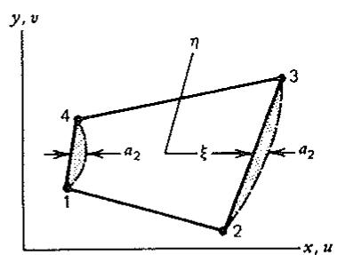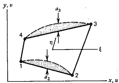The Q6 element is incompatible or nonconforming. For example, as suggested by Fig. 8.3-2, the mode $u = (1 - \eta^{2})a_{2}$ might be activated in one element but not in its neighbors to the left and right, thus producing a gap on one side and an overlap on the other. But incompatible elements are still valid if incompatibilities disappear and a constant-strain state is approached as the mesh is refined. That is, the element is valid if it passes the patch test. If an element of general shape is to pass the patch test, a modified integration scheme is needed; it will be described subsequently. Incompatible elements often yield results of high quality. Interelement gaps and overlaps tend to soften a structure. Softening counters the inherent overstiffness of an assumed-displacement approximation. A good balance of the two effects leads to good results with a coarse mesh. However, the upper-bound nature of the approximation is lost: there is no guarantee that a mesh of incompatible elements will be stiffer than the actual structure. Moreover, in problems that should be independent of Poisson's ratio $\nu$ , a coarse mesh of incompatible elements may display a dependence on $\nu$ . After formulation of element matrices, condensation removes the $a_{i}$ of Eq. 8.3-6. Thus, for the four-node plane element, $a_{1}$ through $a_{4}$ are eliminated, leaving an 8 by 8 condensed matrix [k]. For the special case of a rectangular element, as in Fig. 8.3-1, this condensed [k] is the same as the 8 by 8 [k] produced directly by the displacement field [8.4], $$ \left\{ \begin{array}{l} u \\ v \end{array} \right\} = \left[ \begin{array}{c c c c c c c c} N _ {1} & N _ {x} & N _ {2} & - N _ {x} & N _ {3} & N _ {x} & N _ {4} & - N _ {x} \\ N _ {y} & N _ {1} & - N _ {y} & N _ {2} & N _ {y} & N _ {3} & - N _ {y} & N _ {4} \end{array} \right] \left\{ \begin{array}{l} u _ {1} \\ v _ {1} \\ \vdots \\ u _ {4} \\ v _ {4} \end{array} \right\} \tag {8.3-7} $$ where $N_{1}$ through $\dot{N}_{4}$ are given by Eqs. 6.3-2, and $$ N _ {x} = (1 - \xi^ {2}) \nu \frac {a}{8 b} + (1 - \eta^ {2}) \frac {b}{8 a} \tag {8.3-8} $$ $$ N _ {y} = (1 - \xi^ {2}) \frac {a}{8 b} + (1 - \eta^ {2}) \nu \frac {b}{8 a} $$ 

text_image

y, v η 4 3 a₂ ξ a₂ 1 2 x, u


text_image

y, v a₃ 4 η 3 ξ 1 2 a₃ x, u

Figure 8.3-2. Dashed lines show edge displacements associated with the incompatible modes $u = (1 - \eta^{2})a_{2}$ and $v = (1 - \xi^{2})a_{3}$ in the plane element described by Eqs. 8.3-6. Yet a third way to obtain the same [k] (for a rectangular element) is to begin with the stress field $$ \sigma_ {x} = \beta_ {1} + \beta_ {4} y \quad \sigma_ {y} = \beta_ {2} + \beta_ {5} x \quad \tau_ {x y} = \beta_ {3} \tag {8.3-9} $$ where the $\beta_{i}$ are constants. Using these stress modes, one can invoke the “hybrid” method (Section 8.5), or one can compute the associated displacement field by integration and then proceed in the usual way. Indeed, the latter approach was used very early in finite element history [1.8; see also the discussion cited in Ref. 8.8]. Modified Integration Scheme. The plane and solid elements described by Eq. 8.3-6 pass patch tests only if they are either rectangular or parallelograms and parallelepipeds. A modified integration scheme, here described, corrects this failing [8.3]. Thus modified, the plane element is known as the QM6 element. In the augmented strain-displacement relation $\{\epsilon\} = [\mathbf{B}]\{\mathbf{d}\}$ , let $[\mathbf{B}_a]$ represent the latter columns of [B], that is, the portion of [B] associated with nodeless d.o.f. $a_i$ . Hence, from Eq. 4.1-6, the contribution of the $a_i$ to the consistent element nodal load vector $\{\mathbf{r}_e\}$ is $$ \left\{\mathbf {r} _ {e a} \right\} = - \int_ {V _ {c}} \left[ \mathbf {B} _ {a} \right] ^ {T} \left\{\boldsymbol {\sigma} _ {0} \right\} d V \tag {8.3-10} $$ Imagine that instead of representing initial stresses, $\{\sigma_{0}\}$ represents element stresses produced by nodal displacements $\{d_{r}\}$ on the element boundary. The basic isoparametric element, with neither the $a_{i}$ nor $\{r_{ea}\}$ present, is able to pass a patch test. In other words, when $\{\sigma_{0}\}$ is constant and produced by the “essential” d.o.f. $\{d_{r}\}$ , certain “correct” nodal loads associated with $\{\sigma_{0}\}$ are applied by an element to its nodes. These loads should not be disturbed if incompatible modes are added. Accordingly, in a patch test no additional nodal loads should be associated with the $a_{i}$ . This means that $\{r_{ea}\}$ of Eq. 8.3-10 must vanish when $\{\sigma_{0}\}$ is constant. When $\{\sigma_{0}\}$ is constant, we see that $\{r_{ea}\}$ will be zero if, for plane and solid elements, respectively, $$ \int_ {- 1} ^ {1} \int_ {- 1} ^ {1} \left[ \mathbf {B} _ {a} \right] ^ {T} t J d \xi d \eta = 0 \quad \int_ {- 1} ^ {1} \int_ {- 1} ^ {1} \int_ {- 1} ^ {1} \left[ \mathbf {B} _ {a} \right] ^ {T} J d \xi d \eta d \zeta = 0 \tag {8.3-11} $$ where t is element thickness and J is the Jacobian determinant. For parallelograms of constant thickness and parallelepipeds, t and J are constant and $[B_{a}]$ contains first powers of $\xi$ and $\eta$ (and $\zeta$ for solids), so that Eq. 8.3-11 is satisfied automatically. For elements of general shape, t, J, and $[B_{a}]$ are more complicated functions; Eqs. 8.3-11 are not satisfied and the patch test is failed. But we can “artificially” satisfy Eqs. 8.3-11 as follows. In forming $[B_{a}]$ and integrating, instead of using the correct $[J]^{-1}$ and J at the Gauss quadrature points, use the constant values $[J_{0}]^{-1}$ and $J_{0}$ , where $[J_{0}]$ and $J_{0}$ are the Jacobian matrix and its determinant at $\xi = \eta = \zeta = 0$ . In addition, for plane elements, use $t_{0}$ rather than t if t varies. (If Figs. 6.5-1 and 6.5-2 are adapted to the QM6 element, these adjustments can all be confined to Fig. 6.5-1, in which only columns 9 through 12 of the augmented [B] are affected.) Elements Q6 and QM6 work almost as well as the quadratic element of Eqs. 

text_image

y, v 48 y, v B C 16 A 44 Mesh N = 2 Mesh N = 4 x, u x, u

	Mesh	N=2	N=4
QM6	$v_C$	0.884	0.967
	$\sigma_A$	0.840	0.978
	$\sigma_B$	0.788	0.926
Bilinear	$v_C$	0.498	0.769
	$\sigma_A$	0.558	0.830
	$\sigma_B$	0.457	0.753

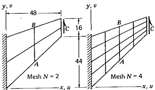
Figure 8.3-3. A plane structure with a uniformly distributed load along the right edge and with $E = 1.0$ , $\nu = 1/3$ . "Bilinear" refers to the element of Eqs. 6.3-2, and $v_{C} =$ deflection at $C$ , $\sigma_{A} =$ maximum stress at $A$ , $\sigma_{B} =$ minimum stress at $B$ , all reported as the ratio of computed value to best-known answer [8.3]. 6.6-1, but only if rectangular. Nevertheless, the QM6 element is considerably more accurate than the bilinear element, as seen in Fig. 8.3-3. (The same problem is solved, using different elements, in Fig. 8.6-2.) Stresses are calculated by using all element d.o.f., including the $a_{i}$ , to evaluate element strains. Calculated stresses are usually more accurate if element nodal loads in $\{r_{e}\}$ that are associated with incompatible modes are set to zero during recovery of the associated d.o.f. $a_{i}$ . # 8.4 ROTATIONAL D.O.F. IN PLANE ELEMENTS The d.o.f. considered are rotations at corner nodes. Such a d.o.f. may also be called a drilling freedom. Its vector representation is normal to the plane of the element. The usual translational d.o.f. at nodes are retained. Thus, a plane triangle with only corner nodes has nine d.o.f. [8.5]. A good reason for use of drilling d.o.f. is found in the modeling of shells as an assembly of flat elements (discussed in detail in Section 12.3). Each element can model bending and stretching actions. Typically, in a general-purpose computer program, d.o.f. allowed at each structure node consist of three displacements and three rotations. Thus drilling d.o.f. are present among structural d.o.f. {D} whether or not they are present among element d.o.f. {d}. If flat shell elements connected to a certain node all happen to be coplanar, but elements do not include drilling d.o.f., then the drilling d.o.f. in {D} at that node is not resisted, and [K] is singular. This difficulty is neatly avoided by including drilling d.o.f. in {d}. Simultaneously, all of the six d.o.f. available at a node are exploited. 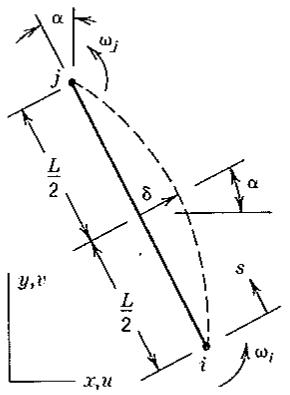In what follows we presume that drilling d.o.f. are associated with parabolic displaced shapes of element sides. In Fig. 8.4-1a, drilling d.o.f. $\omega_{i}$ and $\omega_{j}$ appear at nodes i and j of a typical element side of length L. At midside, $\omega_{i}$ and $\omega_{j}$ produce the edge-normal displacement $\delta$ : $$ \delta = \frac {L}{8} \left(\omega_ {j} - \omega_ {i}\right) \tag {8.4-1} $$ Thus, if $\omega_{i} = \omega_{j}$ , the edge remains straight. If $\omega_{i} \neq \omega_{j}$ , the side assumes a parabolic shape. If $\omega_{i} = -\omega_{j}$ , one can regard $\delta$ as the midspan deflection of a simply 

text_image

α ωj L/2 δ α y,v L/2 s ωi x,u

(a) 

text_image

v₂ ω₂ u₂ 2 ω₃ 3 u₃ v₃ 1 ω₁ u₁ v₁

(b) 

flowchart

```mermaid graph TD v2 --> u2 v2 --> v5 v2 --> 2 v5 --> u5 2 --> 5 5 --> 3 3 --> u3 3 --> v3 v3 --> u6 2 --> 4 4 --> u4 4 --> 6 6 --> 1 1 --> u1 1 --> v1 6 --> v6 v6 --> u6 6 --> v5 v5 --> u5 6 --> v4 v4 --> u4 ```

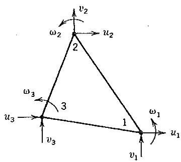
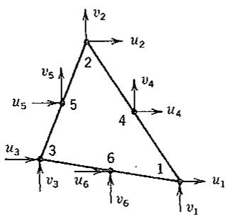
(c) Figure 8.4-1. (a) Side displacement produced by drilling freedoms $\omega_{i}$ and $\omega_{j}$ . (b) A nine-d.o.f. plane triangle. (c) The linear-strain triangle. supported beam of length L under a pure bending moment that produces end rotations $|\omega_{i}| = |\omega_{j}|$ . Extending this beam analogy, imagine that supports of the beam have translational displacement components $u_{i}, v_{i}, u_{j}$ , and $v_{j}$ . Thus edge displacement is the sum of two parts: (a) a straight shape associated with nodal translational d.o.f., and (b) the parabolic shape associated with $\delta$ . The x and y components of $\delta$ are $\delta \cos \alpha$ and $\delta \sin \alpha$ . Therefore, the total displacements u and v of a typical point on the edge are $$ \left\{ \begin{array}{l} u \\ v \end{array} \right\} = \frac {L - s}{L} \left\{ \begin{array}{l} u _ {i} \\ v _ {i} \end{array} \right\} + \frac {s}{L} \left\{ \begin{array}{l} u _ {j} \\ v _ {j} \end{array} \right\} + \frac {(L - s) s}{2 L} \left(\omega_ {j} - \omega_ {i}\right) \left\{ \begin{array}{l} \cos \alpha \\ \sin \alpha \end{array} \right\} \tag {8.4-2} $$ Similar expressions may be written for all other sides of the element. Hence, one can devise shape functions $N_{i}$ for a triangle, a quadrilateral, and so on. In the triangle of Fig. 8.4-1b, contributions to u and v from nodal translations are interpolated linearly over the element, and contributions associated with drilling d.o.f. are interpolated using products of area coordinates, such as $\xi_{1}\xi_{2}$ for $\delta$ on side 1–2. Finally the usual process of element formulation is pursued (Eqs. 4.1-5 and 4.1-6). One can also begin with an element that has straight sides and midside nodes, and convert it to an element that has corner nodes only, each with two translational d.o.f. and one drilling freedom. The conversion process relates midside $\delta$ 's to nodal $\omega$ 's and constrains each edge-tangent displacement component to vary linearly with edge-tangent coordinate s. The element may have any number of sides. As applied to a linear-strain triangle, Fig. 8.4-1c, the transformation procedure is outlined as follows. Consider, for example, side 1–4–2 of the linear-strain triangle, Fig. 8.4-1c. D.o.f. at node 4 are related to d.o.f. at nodes 1 and 2 of the new element, Fig. 8.4-1b, by evaluating Eq. 8.4-2 with s = L/2. With i = 1, j = 2, L cos $\alpha = y_{2} - y_{1}$ , and L sin $\alpha = x_{1} - x_{2}$ , Eq. 8.4-2 yields $$ \left\{ \begin{array}{l} u _ {4} \\ v _ {4} \end{array} \right\} = \frac {1}{2} \left\{ \begin{array}{l} u _ {1} \\ v _ {1} \end{array} \right\} + \frac {1}{2} \left\{ \begin{array}{l} u _ {2} \\ v _ {2} \end{array} \right\} + \frac {\omega_ {2} - \omega_ {1}}{8} \left\{ \begin{array}{l} y _ {2} - y _ {1} \\ x _ {1} - x _ {2} \end{array} \right\} \tag {8.4-3} $$ After doing the same for d.o.f. at nodes 5 and 6, we can relate d.o.f. in Figs. 8.4-1b and 8.4-1c by the transformation $$ \left[ u _ {1} v _ {1} u _ {2} \dots u _ {6} v _ {6} \right] ^ {T} = \left[ \mathrm{T} \right] _ {1 2 \times 9} \left[ u _ {1} v _ {1} \omega_ {1} u _ {2} v _ {2} \omega_ {2} u _ {3} v _ {3} \omega_ {3} \right] ^ {T} \tag {8.4-4} $$ If desired, we can obtain the new element by transforming the stiffness matrix $[k']$ of the linear-strain triangle: $$ \begin{array}{l} \left[ \mathbf {k} \right] = [ \mathbf {T} ] ^ {T} \left[ \mathbf {k} ^ {\prime} \right] [ \mathbf {T} ] \\ 9 \times 9 \end{array} \tag {8.4-5} $$ More efficient coding will result if $[k]$ is formulated directly from shape functions $[N]$ appropriate to the nine-d.o.f. element. These may be obtained by transforming shape functions $[N']$ of the linear-strain triangle: $$ \left\{ \begin{array}{l} u \\ v \end{array} \right\} = \left[ \begin{array}{l} \mathbf {N} ^ {\prime} \\ 2 \times 1 2 \end{array} \right] \left\{ \begin{array}{l} \mathbf {d} ^ {\prime} \\ 1 2 \times 1 \end{array} \right\} = \left[ \begin{array}{l} \mathbf {N} ^ {\prime} \end{array} \right] \left[ \begin{array}{l} \mathbf {T} \end{array} \right] \left\{ \begin{array}{l} \mathbf {d} \\ 9 \times 1 \end{array} \right\} = \left[ \begin{array}{l} \mathbf {N} \\ 2 \times 9 \end{array} \right] \left\{ \begin{array}{l} \mathbf {d} \end{array} \right\} \tag {8.4-6} $$ Shape functions $N_{i}$ in Eq. 8.4-6 agree with those obtained by the procedure described below Eq. 8.4-2. Deformations are everywhere zero if all nodal rotations in the mesh have the same value. This mechanism can be suppressed by prescribing the value of one nodal rotation in the mesh, for example, by setting $\omega_{1} = 0$ . The true rotation at a node i is defined as $$ \theta_ {i} = \frac {1}{2} (v _ {, x} - u _ {, y}) _ {i} \tag {8.4-7} $$ For rigid-body rotation in the plane of the element, $\theta_{i} = \omega_{i}$ . Otherwise, equality may not prevail [8.5]. Interelement continuity of true rotations is not in general provided, nor is it necessary for proper convergence of the finite element solution. A plane quadrilateral with drilling d.o.f. is described in [8.37]. It incorporates various improvements, including a device to control the aforementioned mechanism. This device is summarized as follows. Let the strain energy in each element be augmented by $U_{\omega}$ , $$ U _ {\omega} ^ {\prime} = \frac {1}{2} V _ {e} G (2 \gamma) \left(\theta_ {0} - \frac {1}{n} \sum_ {i = 1} ^ {n} \omega_ {i}\right) ^ {2} \tag {8.4-8} $$ where $V_{e} = \text{element volume}$ , G = shear modulus, $\gamma = \text{dimensionless constant}$ ( $\gamma = 10^{-6}$ is recommended), $\theta_{0} = (v_{,x} - u_{,y})_{0}/2$ is the rotation at the element center, and n = number of nodes where rotational d.o.f. $\omega_{i}$ are used. By inserting shape functions, we can write the parenthetic expression in Eq. 8.4-8 in matrix format; that is, $(\cdots) = \lfloor Q \rfloor \{d\}$ , where $\lfloor Q \rfloor$ is a row matrix. Hence $$ U _ {\omega} = \frac {1}{2} \left\{\mathbf {d} \right\} ^ {T} \left[ \mathbf {k} _ {\omega} \right] \left\{\mathbf {d} \right\} \quad \text { in which } \quad \left[ \mathbf {k} _ {\omega} \right] = 2 \gamma V _ {e} G \left[ \mathbf {Q} \right] ^ {T} \left[ \mathbf {Q} \right] \tag {8.4-9} $$ where $[k_{\omega}]$ is a rank 1 “stabilization matrix” that is added to the existing element stiffness matrix. Matrix $[k_{\omega}]$ has no effect on the ability of the element to represent constant-strain states and rigid-body modes. Numerical examples are reported in Fig. 8.6-2 and in Refs. 8.5, 8.6, and 8.37. # 8.5 ASSUMED-STRESS HYBRID FORMULATION The assumed-stress hybrid method is a way of formulating a stiffness matrix by use of independent assumptions of (a) an equilibrium stress field within the element, and (b) interelement-compatible displacement modes on the element boundary. Mathematically, the method can be stated as a modified complementary energy principle. The principle of stationary complementary energy states that: among all stress fields that satisfy the differential equations of equilibrium, the stress field that also satisfies compatibility conditions makes the complementary energy stationary with respect to small variations of stress. For a linearly elastic material, strain energy per unit volume can be written as $$ \begin{array}{l} U _ {0} = \frac {1}{2} \{\boldsymbol {\epsilon} \} ^ {T} [ \mathrm{E} ] \{\boldsymbol {\epsilon} \} \quad \text { or as } \quad U _ {0} = \frac {1}{2} \{\boldsymbol {\sigma} \} ^ {T} [ \mathrm{E} ] ^ {- 1} \{\boldsymbol {\sigma} \} \tag {8.5-1} \\ (\text { potential energy }) \quad \text {(complementary energy)} \\ \end{array} $$ Starting with an expression for $U_{0}$ , one can write various functionals. The functional for potential energy is $\Pi_{p}$ , Eq. 4.1-1, which yields the stiffness matrix of an element based on an assumed displacement field. Analogously, one can write a complementary energy functional that yields the stiffness matrix of an assumed-stress hybrid element [8.7]. Rather than discuss the functional, we consider the following more direct method, which is the method by which assumed-stress hybrid elements were first derived [8.8]. Although the hybrid method is general, the discussion that follows is oriented toward plane problems without body forces. One begins with a stress field that satisfies the differential equations of equilibrium, Eqs. 1.6-2 and 1.6-4. Symbolically, $$ \{\sigma \} = [ \mathbf {P} ] \{\beta \} \tag {8.5-2} $$ where, for plane problems, $\{\sigma\} = \left[\sigma_x - \sigma_y - \tau_{xy}\right]^T$ , and $\{\beta\}$ contains constants $\beta_i$ that are yet to be determined. Equations 8.3-9 are a $5-\beta$ example of such an equilibrium stress field. From Eqs. 8.5-1 and 8.5-2, the complementary strain energy in an element of volume $V_e$ is $$ U = \int_ {V _ {e}} U _ {0} d V = \frac {1}{2} \{\boldsymbol {\beta} \} ^ {T} [ \mathbf {H} ] \{\boldsymbol {\beta} \} \tag {8.5-3} $$ where $$ [ \mathbf {H} ] = \int_ {V _ {e}} [ \mathbf {P} ] ^ {T} [ \mathbf {E} ] ^ {- 1} [ \mathbf {P} ] d V \tag {8.5-4} $$ Let $\{\Phi\}$ represent tractions at the element boundary $S_{e}$ , obtained by evaluating Eq. 8.5-2 on the boundary. Also let boundary displacements $\{\mathbf{u}_{b}\}$ be interpolated from nodal d.o.f. $\{\mathbf{d}\}$ . (An example will follow.) Thus $$ \{\Phi \} = [ \mathbf {R} ] \{\beta \} \quad \text { and } \quad \{\mathbf {u} _ {b} \} = [ \mathbf {L} ] \{\mathbf {d} \} \tag {8.5-5} $$ The total complementary energy in the element is U minus work done by tractions $\{\Phi\}$ in moving through displacements $\{u_{b}\}$ ; that is, $$ \Pi_ {c} = U - \int_ {S _ {e}} \{\Phi \} ^ {T} \{\mathbf {u} _ {b} \} d S = \frac {1}{2} \{\boldsymbol {\beta} \} ^ {T} [ \mathbf {H} ] \{\boldsymbol {\beta} \} - \{\boldsymbol {\beta} \} ^ {T} [ \mathbf {G} ] \{\mathbf {d} \} \tag {8.5-6} $$ where $$ [ \mathbf {G} ] = \int_ {S _ {e}} [ \mathbf {R} ] ^ {T} [ \mathbf {L} ] d S \tag {8.5-7} $$ Making $\Pi_{c}$ stationary with respect to variations of stress, we write $$ \frac {\partial \Pi_ {c}}{\partial \beta_ {i}} = 0 \quad \text { for } \quad i = 1, 2, \dots , n \quad \text { or } \quad \left\{\frac {\partial \Pi_ {c}}{\partial \beta} \right\} = \{0 \} \tag {8.5-8} $$ from which $$ [ \mathbf {H} ] \{\boldsymbol {\beta} \} = [ \mathbf {G} ] \{\mathbf {d} \} \quad \text { or } \quad \{\boldsymbol {\beta} \} = [ \mathbf {H} ] ^ {- 1} [ \mathbf {G} ] \{\mathbf {d} \} \tag {8.5-9} $$ At this point one can say that we have asked for the stress field within an element when displacements on its boundary are prescribed, and answered by finding values of $\{\beta\}$ that define the best stress field $\{\sigma\}$ that is contained in the approximation $\{\sigma\} = [P]\{\beta\}$ . Substitution of $\{\beta\}$ from Eq. 8.5-9 into Eq. 8.5-3 yields $$ U = \frac {1}{2} \{\mathbf {d} \} ^ {T} [ \mathbf {k} ] \{\mathbf {d} \}, \quad \text { where } \quad [ \mathbf {k} ] = [ \mathbf {G} ] ^ {T} [ \mathbf {H} ] ^ {- 1} [ \mathbf {G} ] \tag {8.5-10} $$ in which $[k]$ is recognized as a stiffness matrix because its form matches that of Eq. 4.1-10. Example. Consider a typical straight edge $ij$ of a plane element, Fig. 8.5-1a. Tractions $\Phi_x$ and $\Phi_y$ are related to stresses $\sigma_x$ , $\sigma_y$ , and $\tau_{xy}$ by direction cosines $\ell$ and $m$ of the outward normal to the edge. From Eq. 1.6-3, $$ \begin{array}{l} \Phi_ {x} = \ell \sigma_ {x} + m \tau_ {x y} \quad \text { where } \quad \ell = \cos \alpha = (y _ {j} - y _ {i}) / L _ {i j} \tag {8.5-11} \\ \Phi_ {y} = \ell \tau_ {x y} + m \sigma_ {y} \quad \text { where } \quad m = \sin \alpha = (x _ {i} - x _ {j}) / L _ {i j} \\ \end{array} $$ For the particular case of a 5- $\beta$ rectangular element, Eqs. 8.3-9 and Fig. 8.5-1b, arrays [P] and [R] are $$ [ \mathbf {P} ] = \left[ \begin{array}{l l l l l} 1 & 0 & 0 & y & 0 \\ 0 & 1 & 0 & 0 & x \\ 0 & 0 & 1 & 0 & 0 \end{array} \right] \quad \text { and } \quad [ \mathbf {R} ] = \left[ \begin{array}{l l l l l} 0 & 0 & - 1 & 0 & 0 \\ 0 & - 1 & 0 & 0 & - x \\ 1 & 0 & 0 & y & 0 \\ 0 & 0 & 1 & 0 & 0 \\ 0 & 0 & 1 & 0 & 0 \\ 0 & 1 & 0 & 0 \cdot & x \\ - 1 & 0 & 0 & - y & 0 \\ 0 & 0 & - 1 & 0 & 0 \end{array} \right] \tag {8.5-12} $$ where [R] is obtained from [P] and Eq. 8.5-11. The first two rows of [R] pertain to $\Phi_x$ and $\Phi_y$ along side 1-2 (where $\ell = 0$ and $m = -1$ ), the third and fourth rows pertain to $\Phi_x$ and $\Phi_y$ along side 2-3 (where $\ell = 1$ and $m = 0$ ), and so on. Matrix [L] of Eq. 8.5-5 is 8 by 8 for the element of Fig. 8.5-1b, and relates $u$ and $v$ displacement components along all four edges to nodal d.o.f. {d}. That is,