text_image
y,v
α
j
Φy
σx ← τxy → Φx
σy
Lij
i
s
α
x,u
(a)
text_image
y,v
a
a
4
3
b
x,u
b
1
2
(b)
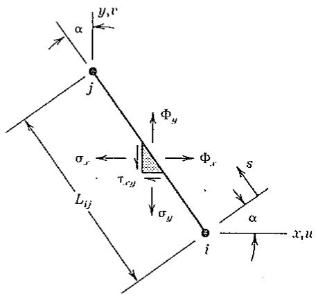
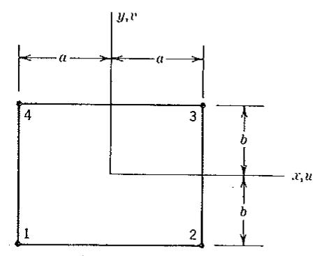
Figure 8.5-1. (a) Stresses and surface tractions at a typical edge ij. (b) A rectangular element.
$$
\left[ \begin{array}{l l l l l} u _ {1 2} & v _ {1 2} & u _ {2 3} \cdot \cdot \cdot u _ {4 1} & v _ {4 1} \end{array} \right] ^ {T} = [ \mathrm{L} ] \left[ \begin{array}{l l l l} u _ {1} & v _ {1} \cdot \cdot \cdot u _ {4} & v _ {4} \end{array} \right] ^ {T} \tag {8.5-13}
$$
If $\mu$ and $\nu$ along an edge are linearly interpolated from nodal d.o.f. on that edge, the rows of [L] are
$$
\text { row 1: } \quad \frac {a - x}{2 a}, 0, \frac {a + x}{2 a}, 0, 0, 0, 0, 0 \tag {8.5-14}
$$
$$
\text { row 2: } \quad 0, \frac {a - x}{2 a}, 0, \frac {a + x}{2 a}, 0, 0, 0, 0
$$
and so on. All ingredients are now at hand: the element stiffness matrix is obtained by application of Eqs. 8.5-4, 8.5-7, and 8.5-10. In integration of Eq. 8.5-4, $dV$ becomes $t \, dA = t \, dx \, dy$ , where $t$ is the element thickness. In integration of Eq. 8.5-7, $dS = t \, ds$ , where $ds = dx$ or $ds = dy$ for sides parallel to $x$ and $y$ axes, respectively. Terms that contain $x$ are integrated from $-a$ to $+a$ and terms that contain $y$ are integrated from $-b$ to $+b$ .
Remarks. After $\{d\}$ is known, element stresses are recovered by use of Eqs. 8.5-2 and 8.5-9. Thus
$$
\{\sigma \} = [ \mathrm{P} ] [ \mathrm{H} ] ^ {- 1} [ \mathrm{G} ] \{\mathrm{d} \} \tag {8.5-15}
$$
Assumed-stress hybrid elements can be joined to displacement-based elements because both use displacement quantities as nodal d.o.f. The user of a computer program may be unaware that some of its elements are hybrid elements.
Assumed-stress hybrid elements become stiffer as $\{\beta\}$ grows—that is, as more terms are added to the stress expansion. They usually become more flexible as element edges are permitted more complicated displacement patterns. No bound can be set: we cannot say in general that a mesh of hybrid elements will be too stiff or too flexible. If $\{\sigma\} = [P]\{\beta\}$ is not a complete polynomial, the element will not be geometrically isotropic. For example, the stress field described by [P] of Eq. 8.5-12 is not complete. A complete linear stress field in the plane is
$$
\left\{ \begin{array}{l} \sigma_ {x} \\ \sigma_ {y} \\ \tau_ {x y} \end{array} \right\} = \left[ \begin{array}{c c c c c c c} 1 & 0 & 0 & y & 0 & x & 0 \\ 0 & 1 & 0 & 0 & x & 0 & y \\ 0 & 0 & 1 & 0 & 0 & - y & - x \end{array} \right] \left\{ \begin{array}{l} \beta_ {1} \\ \beta_ {2} \\ \vdots \\ \beta_ {7} \end{array} \right\} \tag {8.5-16}
$$
This field contains seven $\beta_{i}$ rather than nine in order to satisfy the differential equations of equilibrium. If used with linear edge displacements (e.g., Eq. 8.5-14), the $7-\beta$ element has eight displacement d.o.f. but is stiffer than a $5-\beta$ element having the same eight displacement d.o.f.
It is possible to relax the requirement that stresses satisfy the differential equations of equilibrium a priori. Procedures suggested by Wolf [8.9] and Pian [8.10] use a functional in which displacements within the element act as Lagrange multipliers of the differential equations of equilibrium. Equilibrium is then satisfied in an average sense rather than at every point.
# 8.6 A PLANE HYBRID TRIANGLE WITH ROTATIONAL D.O.F.
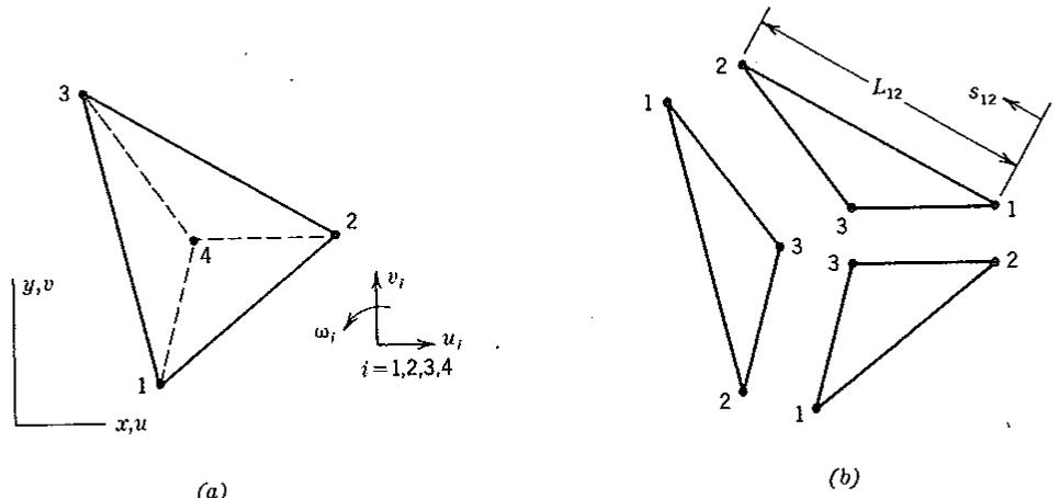
Hybrid element theory (Section 8.5) and “drilling” d.o.f. (Section 8.4) are combined in the element here described [8.11]. It is a triangle built of three subtriangles. The final macroelement is a nine-d.o.f. triangle (Fig. 8.6-1). The same element can be obtained by standard displacement theory, as explained in the following.
Basic Triangular Subelement. Stresses are assumed constant: $\sigma_{x} = \beta_{1}$ , $\sigma_{y} = \beta_{2}$ , and $\tau_{xy} = \beta_{3}$ . Thus [P] is a unit matrix, and Eq. 8.5-4 yields
$$
\left[ \mathbf {H} \right] _ {3 \times 3} = A t [ \mathbf {E} ] ^ {- 1} \quad \text { and } \quad \left[ \mathbf {H} \right] ^ {- 1} = \frac {1}{A t} [ \mathbf {E} ] \tag {8.6-1}
$$
where $A =$ subelement area and $t =$ subelement thickness.
where $A =$ subcontinent area and $\mathbf{A} = \mathbf{A}_0$ . Matrix [R] is 6 by 3 and is formed from boundary tractions $\Phi_x = \ell \beta_1 + m\beta_3$ and $\Phi_y = \ell \beta_3 + m\beta_2$ . Direction cosines $\ell$ and $m$ are given by Eq. 8.5-11. For
(a)
Figure 8.6-1. (a) Triangular macroelement built of three subtriangles. D.o.f. of a typical node i are shown. (b) Node labels for the subtriangles.
example, terms in the first two rows of [R] pertain to side 1–2 of the subelement and are
$$
\text { row 1: } \quad (y _ {2} - y _ {1}) / L _ {1 2}, 0, (x _ {1} - x _ {2}) / L _ {1 2}
$$
$$
\text { row 2: } \quad 0, (x _ {1} - x _ {2}) / L _ {1 2}, (y _ {2} - y _ {1}) / L _ {1 2} \tag {8.6-2}
$$
Boundary displacements and nodal d.o.f. are related via matrix [L]. The relationship resembles Eq. 8.5-13, but involves one less side, one less node, and three d.o.f. per node. Rows of [L] are written by application of Eq. 8.4-2. For example, the first row of [L] expresses the relation
$$
u _ {1 2} = \frac {L _ {1 2} - s _ {1 2}}{L _ {1 2}} u _ {1} + \frac {s _ {1 2}}{L _ {1 2}} u _ {2} + \frac {y _ {2} - y _ {1}}{L _ {1 2}} \frac {(L _ {1 2} - s _ {1 2}) s _ {1 2}}{2 L _ {1 2}} (\omega_ {2} - \omega_ {1}) \tag {8.6-3}
$$
where $s_{12}$ is an edge-tangent coordinate, Fig. 8.6-1b.
When matrix [G] of Eq. 8.5-7 is computed, $dS = t ds_{ij}$ and limits of integration are from 0 to $L_{ij}$ , where $L_{ij}$ is $L_{12}$ , $L_{23}$ , or $L_{31}$ for the respective element sides. Let nodal d.o.f. have the ordering $\{\mathbf{d}\} = \left[u_1 \quad v_1 \quad \omega_1 \quad u_2 \quad v_2 \quad \omega_2 \quad u_3 \quad v_3 \quad \omega_3\right]^T$ . Then, in partitioned form, [G] is
$$
\left[ \begin{array}{l} \mathbf {G} \\ 3 \times 9 \end{array} \right] = \left[ \begin{array}{l l l} \mathbf {G} _ {A} & \mathbf {G} _ {B} & \mathbf {G} _ {C} \end{array} \right] \tag {8.6-4}
$$
where, with $y_{ij} = y_i - y_j$ and $x_{ij} = x_i - x_j$ ,
$$
\left[ \mathrm{G} _ {A} \right] = \frac {t}{1 2} \left[ \begin{array}{c c c} 6 y _ {2 3} & 0 & y _ {3 1} ^ {2} - y _ {1 2} ^ {2} \\ 0 & 6 x _ {3 2} & x _ {1 3} ^ {2} - x _ {2 1} ^ {2} \\ 6 x _ {3 2} & 6 y _ {2 3} & 2 \left(x _ {1 3} y _ {3 1} - x _ {2 1} y _ {1 2}\right) \end{array} \right] \tag {8.6-5}
$$
Submatrices $[G_{B}]$ and $[G_{C}]$ are obtained from $[G_{A}]$ by advancing the subscripts by 1 and 2 respectively around the loop 1–2–3; for example, $x_{32}$ in $[G_{A}]$ becomes $x_{13}$ in $[G_{B}]$ and $x_{21}$ in $[G_{C}]$ .
The foregoing triangular subelement can also be generated from an assumed displacement field: one uses the 2 by 9 matrix [N] of Eq. 8.4-6, and integrates $[B]^{T}[E][B]$ by using a single Gauss point at the centroid of the element (or subelement, in the present context).
Macroelement. The composite element—that is, the macroelement, Fig. 8.6-1a—is formed by combining three of the foregoing subelements. Node 4 is at the centroid of the macroelement, that is, at
$$
x _ {4} = \frac {1}{3} (x _ {1} + x _ {2} + x _ {3}) \quad \text { and } \quad y _ {4} = \frac {1}{3} (y _ {1} + y _ {2} + y _ {3}) \tag {8.6-6}
$$
D.o.f. at node 4 can be eliminated by static condensation, leaving a three-node element having nine d.o.f.
However, such an element is a bit too flexible in many problems. Accordingly, prior to condensation, the rotational d.o.f. at node 4 is constrained to be the average of rotational d.o.f. at nodes 1, 2, and 3. This is accomplished by first transforming the 12 by 12 matrix [k] so that it operates on nodal d.o.f. {d} in which $\omega_{4r}$ replaces $\omega_{4}$ , where
text_image
y,v
48
B
16
C
A
44
Mesh N = 2
x,u
y,v
B
C
A
Mesh N = 4
x,u
| Mesh | N=2 | N=4 |
| Equation8.4-5 | $v_{C}$ | 0.840 | 0.950 |
| $\sigma_{A}$ | 0.682 | 0.878 |
| $\sigma_{B}$ | 0.730 | 0.856 |
| Figure8.6-1 | $v_{C}$ | 0.900 | 0.969 |
| $\sigma_{A}$ | 0.746 | 0.909 |
| $\sigma_{B}$ | 0.917 | 0.882 |
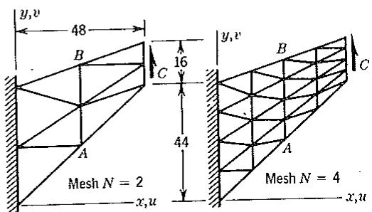
Figure 8.6-2. A plane structure with a uniformly distributed load along the right edge and with $E = 1.0$ , $\nu = 1/3$ . Results displayed are obtained from elements that have drilling d.o.f. “Equation 8.4-5” refers to the nine-d.o.f. displacement-based element obtainable from the linear-strain triangle [8.5]. “Figure 8.6-1” refers to the composite element with constant-stress subtriangles and $\omega_4 = (\omega_1 + \omega_2 + \omega_3)/3$ . Here $v_C =$ deflection at $C$ , $\sigma_A =$ maximum stress at $A$ , $\sigma_B =$ minimum stress at $B$ , all reported as the ratio of computed value to best-known answer.
$$
\omega_ {4 r} = \omega_ {4} - \frac {1}{3} (\omega_ {1} + \omega_ {2} + \omega_ {3}) \tag {8.6-7}
$$
Here $\omega_{4r}$ is the rotational d.o.f. at node 4 relative to the average of the three vertex rotational d.o.f. The constraint is $\omega_{4r} = 0$ , which is enforced by striking out the row and column of the transformed [k] associated with $\omega_{4r}$ . This leaves an 11 by 11 stiffness matrix, from which $u_{4}$ and $v_{4}$ are eliminated by static condensation.
The resulting nine-d.o.f. element is geometrically isotropic and has rank 5, corresponding to three rigid-body motions and the mechanism in which all nodal rotations are the same. The patch test is passed. Numerical results are reported as the “Fig. 8.6-1” entries in Fig. 8.6-2. The same problem is solved, using different elements, in Fig. 8.3-3.
# 8.7 USER-DEFINED ELEMENTS. ELASTIC KERNEL
The user of a computer program may wish to supply an element of a type not provided in the program. If all stiffness coefficients $k_{ij}$ of the new element are supplied directly, rather than as the output of a tested algorithm, there is substantial risk of introducing numerical error. In the following we explain a procedure whereby only some of the $k_{ij}$ need be supplied, and we comment on why this procedure is effective in avoiding the possible error.
First, the element stiffness equation $[\mathbf{k}]\{\mathbf{d}\} = \{\mathbf{r}\}$ is partitioned,
$$
\left[ \begin{array}{l l} \mathbf {k} _ {R R} & \mathbf {k} _ {R E} \\ \mathbf {k} _ {R E} ^ {T} & \mathbf {k} _ {E E} \end{array} \right] \left\{ \begin{array}{l} \mathbf {d} _ {R} \\ \mathbf {d} _ {E} \end{array} \right\} = \left\{ \begin{array}{l} \mathbf {r} _ {R} \\ \mathbf {r} _ {E} \end{array} \right\} \tag {8.7-1}
$$
in which d.o.f. $\{d_{R}\}$ are used to define rigid-body motion of the element and d.o.f. $\{d_{E}\}$ are used to define straining modes (an example follows). For any element, there is more than one way to partition $\{d\}$ into $\{d_{R}\}$ and $\{d_{E}\}$ . We wish to describe how the stiffness matrix $[k_{EE}]$ of an element that is fully (but not redundantly) restrained from rigid-body motion ( $\{d_{R}\} = \{0\}$ ) can be converted to a complete stiffness matrix [k], ready for assembly into the structure.
The lower partition of Eq. 8.7-1 is solved for $\{d_{E}\}$ . Also, this expression for $\{d_{E}\}$ is substituted into the upper partition. Thus
$$
\left[ \begin{array}{c c} \left(\mathbf {k} _ {R R} - \mathbf {k} _ {R E} \mathbf {k} _ {E E} ^ {- 1} \mathbf {k} _ {R E} ^ {T}\right) & \mathbf {k} _ {R E} \mathbf {k} _ {E E} ^ {- 1} \\ - \mathbf {k} _ {E E} ^ {- 1} \mathbf {k} _ {R E} ^ {T} & \mathbf {k} _ {E E} ^ {- 1} \end{array} \right] \left\{ \begin{array}{l} \mathbf {d} _ {R} \\ \mathbf {r} _ {E} \end{array} \right\} = \left\{ \begin{array}{l} \mathbf {r} _ {R} \\ \mathbf {d} _ {E} \end{array} \right\} \tag {8.7-2}
$$
Matrix $[\mathbf{k}_{EE}]$ is symmetric and is invertible because rigid-body motion is prevented. If there is no elastic distortion, then $\{\mathbf{r}_E\} = \{\mathbf{0}\}$ and, therefore,
$$
- \left[ \mathbf {k} _ {E E} \right] ^ {- 1} \left[ \mathbf {k} _ {R E} \right] ^ {T} \left\{\mathbf {d} _ {R} \right\} = \left\{\mathbf {d} _ {E} \right\} \tag {8.7-3}
$$
With $\{r_{E}\}=\{0\}$ , only rigid-body motion is possible. We also know that in rigid-body motion nodal d.o.f. are related strictly by kinematics, expressed by a matrix [T] of element dimensions:
$$
\{\mathbf {d} _ {E} \} = [ \mathbf {T} ] \{\mathbf {d} _ {R} \} \tag {8.7-4}
$$
Typically $\{d_{E}\}$ contains more d.o.f. than $\{d_{R}\}$ , in which case [T] contains more rows than columns. Because Eqs. 8.7-3 and 8.7-4 must be true for any $\{d_{R}\}$ , we thus conclude, by comparison, that
$$
[ \mathbf {k} _ {R E} ] ^ {T} = - [ \mathbf {k} _ {E E} ] [ \mathbf {T} ] \tag {8.7-5}
$$
Next imagine that $\{\mathbf{r}_E\} \neq \{\mathbf{0}\}$ . Then, because $\{\mathbf{d}_R\}$ contains only enough d.o.f. to prevent rigid-body motion, $\{\mathbf{r}_R\}$ can be computed from $\{\mathbf{r}_E\}$ entirely by equations of statics, independently of $\{\mathbf{d}_R\}$ . Accordingly, the coefficient of $\{\mathbf{d}_R\}$ in the upper partition of Eq. 8.7-2 must vanish. From this and Eq. 8.7-5 we obtain
$$
[ \mathbf {k} _ {R R} ] = [ \mathbf {k} _ {R E} ] [ \mathbf {k} _ {E E} ] ^ {- 1} [ \mathbf {k} _ {R E} ] ^ {T} = [ \mathbf {T} ] ^ {T} [ \mathbf {k} _ {E E} ] [ \mathbf {T} ] \tag {8.7-6}
$$
The stiffness matrix that operates on all nodal d.o.f., $\{\mathbf{d}\} = \lfloor \mathbf{d}_R - \mathbf{d}_E\rfloor^T$ , is therefore
$$
[ \mathbf {k} ] = \left[ \begin{array}{c c} \mathbf {T} ^ {T} \mathbf {k} _ {E E} \mathbf {T} & - \mathbf {T} ^ {T} \mathbf {k} _ {E E} \\ - \mathbf {k} _ {E E} \mathbf {T} & \mathbf {k} _ {E E} \end{array} \right] \tag {8.7-7}
$$
Matrix $[\mathbf{k}_{EE}]$ is called the elastic kernel.
The user must supply $[k_{EE}]$ (or supply and then invert the flexibility matrix $[k_{EE}]^{-1}$ ) and [T] to the computer program. Equation 8.7-7 then produces a [k] that requires no force to produce rigid-body motion. If the user were required to prescribe the entire [k], the individual $k_{ij}$ would have to be of full computer-word accuracy to avoid the possibility of introducing serious errors (Section 18.2). By use of Eq. 8.7-7, slight errors in the $(k_{EE})_{ij}$ produce only slight defects in elastic response; they do not cause rigid-body motion to be misrepresented.
Example. Consider the standard beam element of Fig. 4.2-2. Let the element be fixed at its left end, so that $\{\mathbf{d}_R\} = \lfloor w_1 - \theta_1 \rfloor^T$ . Then $\{\mathbf{d}_E\} = \lfloor w_2 - \theta_2 \rfloor^T$ . From Eq. 4.2-4, the curvature
$$
w _ {, x x} = \left\lfloor \frac {6}{L ^ {2}} - \frac {1 2 x}{L ^ {3}} \quad - \frac {2}{L} + \frac {6 x}{L ^ {2}} \right\rfloor \left\{\mathbf {d} _ {E} \right\} \tag {8.7-8}
$$
is used to construct $[\mathbf{k}_{EE}]$ , which is found to be the lower right 2 by 2 submatrix in Eq. 4.2-5. Equation 8.7-4 becomes
$$
\left\{ \begin{array}{l} w _ {2} \\ \theta_ {2} \end{array} \right\} = [ \mathrm{T} ] \left\{ \begin{array}{l} w _ {1} \\ \theta_ {1} \end{array} \right\}, \quad \text { where } \quad [ \mathrm{T} ] = \left[ \begin{array}{l l} 1 & L \\ 0 & 1 \end{array} \right] \tag {8.7-9}
$$
Equation 8.7-7 then yields [k] of Eq. 4.2-5.
# 8.8 HIGHER DERIVATIVES AS NODAL D.O.F.
For the following discussion we define “essential” d.o.f. as the particular nodal d.o.f. needed to achieve the minimally-acceptable degree of interelement compatibility. These are the familiar nodal d.o.f. used in Chapters 1 through 7: for example, $u_{i}$ and $v_{i}$ for bars and plane elements, $w_{i}$ and $\theta_{i}$ for beam elements. We define a “higher derivative” as one that is not needed to define interelement compatibility. Thus, in the stretching of a bar or in plane stress, all derivatives of u and v would be considered “higher.” In the bending of a beam or a thin plate, higher derivatives are second and greater derivatives of lateral displacement. When used as nodal d.o.f., higher derivatives are also called “extra” or “excessive.”
Elements with higher-derivative d.o.f. have certain advantages. They are based on fields having many generalized coordinates, so they provide good accuracy in a coarse mesh. Strains (or curvatures) needed in the calculation of stresses (or bending moments) appear in $\{\mathbf{D}\}$ . Thus, being primary unknowns, strains may be computed more accurately than the conventionally computed strains $\{\epsilon\} = [\mathbf{B}]\{\mathbf{d}\}$ , which invoke difference operations on essential d.o.f. $\{\mathbf{d}\}$ . Moreover, the extra d.o.f. are available at nodes, the very place where conventional strains $\{\epsilon\} = [\mathbf{B}]\{\mathbf{d}\}$ are likely to be least accurate.
However, elements having higher-derivative d.o.f. are sometimes awkward to use. At an elastic–plastic boundary, or where there is an abrupt change in stiffness or material properties, continuity of higher derivative d.o.f. must not be enforced. For example, if two beam elements of different stiffness are joined, they have the same moment but different curvature at the node they share. A maneuver appropriate to such a circumstance is to release the curvature d.o.f. in one of the elements before assembly (Section 8.1). But, by doing so, we reduce the benefit of these d.o.f. where it is most needed—near a high-stress gradient.
Release of higher-derivative d.o.f. is again required and the benefit of these d.o.f. is again reduced if elements with derivative d.o.f. must be used in combination with elements that have only essential nodal d.o.f. Indeed, many computer programs allow up to six d.o.f. per node (three translations and three rotations) and so may be unable to accommodate a higher-order element without basic changes.
Boundary conditions may become awkward because the physical meaning of higher-derivative d.o.f. and their associated nodal loads is obscure. For example, if a plane element includes derivatives $u_{,x}, u_{,y}, v_{,x}$ , and $v_{,y}$ as nodal d.o.f., a stress-free boundary dictates a constraint relation among these d.o.f. but does not dictate the numerical value of any of them.
In summary, higher-derivative d.o.f. tend to make the finite element method
awkward in application to problems for which it is most powerful—to structures built of different element types and involving thickness changes, stiffeners, and parts that join with sharp angles instead of smooth curves.
# 8.9 FRACTURE MECHANICS.
# SINGULARITY ELEMENTS
Fracture mechanics deals with the conditions under which a body can fail owing to the propagation of an existing crack of macroscopic size $[8.12]$ . In analysis, one might ask for the load that will produce failure when a crack of known size is present, or for the allowable size of a crack when a known load must be sustained.
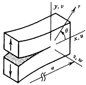
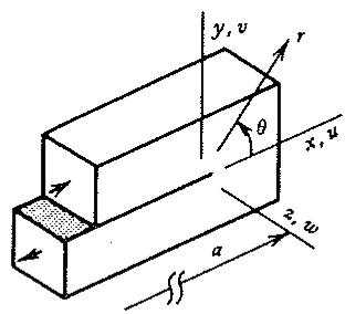
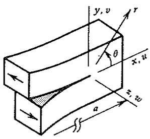
Consider an arbitrarily loaded body that contains a crack. By isolating material in the immediate neighborhood of a crack tip, one can identify the three possible deformation modes shown in Fig. 8.9-1. These modes may appear singly or in arbitrary combination. Formulas exist for stresses and displacements in the immediate neighborhood of a crack tip. For example, if the crack is Mode I and the material is linearly elastic and isotropic, the y-direction stress and displacement are.
$$
\sigma_ {y} = \frac {K _ {\mathrm{I}}}{(2 \pi r) ^ {1 / 2}} \left(\cos \frac {\theta}{2}\right) \left[ 1 + \sin \frac {\theta}{2} \sin \frac {3 \theta}{2} \right] \tag {8.9-1}
$$
$$
v = \frac {(2 \pi r) ^ {1 / 2}}{8 G \pi} K _ {\mathrm{I}} \left[ (2 \kappa + 1) \sin \frac {\theta}{2} - \sin \frac {3 \theta}{2} \right] \tag {8.9-2}
$$
where $G =$ shear modulus, and with $\nu =$ Poisson's ratio,
$$
\kappa = 3 - 4 \nu \quad (\text { plane strain }) \quad \text { or } \quad \kappa = \frac {3 - \nu}{1 + \nu} \quad (\text { plane stress }) \tag {8.9-3}
$$
Here $K_{I}$ is called the stress intensity factor for Mode I. It can be defined as
$$
K _ {\mathrm{I}} = \lim _ {r \rightarrow 0} \left[ \sigma_ {y} (2 \pi r) ^ {1 / 2} \right] \quad \text { for } \quad \theta = 0 \tag {8.9-4}
$$
text_image
y, v
r
θ
x, u
a, w
a
Mode I (opening)
text_image
y, v
r
θ
x, u
z, w
a
Mode II (sliding)
text_image
y, v
r
θ
x, u
z, u
a
Mode III (tearing)
Figure 8.9-1. Deformation modes in the immediate neighborhood of a crack tip.
text_image
σ
2a
σ
2c
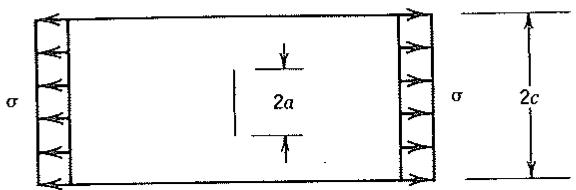
Figure 8.9-2. Flat plate with a central crack of width 2a. Tensile stress $\sigma$ is uniform well away from the crack.
A stress intensity factor is not a stress concentration factor: a stress intensity factor pertains to a singularity in the stress field, whereas a stress concentration factor pertains to geometries that do not produce infinite stresses. Nevertheless, two factors are analogous in that results are known and tabulated for several geometries and loadings $[8.13]$ . For example, in Fig. 8.9-2,
$$
K _ {1} = \sigma (\pi a) ^ {1 / 2} \frac {1 - 0 . 5 (a / c) + 0 . 3 2 6 (a / c) ^ {2}}{\left[ 1 - (a / c) \right] ^ {1 / 2}} \tag {8.9-5}
$$
There is a value of $K_{\mathrm{I}}$ denoted by $K_{\mathrm{IC}}$ and called fracture toughness. $K_{\mathrm{IC}}$ can be regarded as a material constant for which data are known. If $K_{\mathrm{I}} = K_{\mathrm{IC}}$ in Eq. 8.9-5, a "critical" condition exists—that is, fracture impends. Thus, given $K_{\mathrm{IC}}$ , $a$ , and $c$ , one can solve for the critical value of $\sigma$ . Or, given $K_{\mathrm{IC}}$ , $\sigma$ , and $c$ , one can solve for the critical value of crack length $2a$ . In Eq. 8.9-5, note that $\sigma$ is stress on the gross cross-sectional area $2ct$ , not stress on the net area $2(c - a)t$ .
For complicated geometries and loadings, formulas such as Eq. 8.9-5 are not tabulated. A substitute relation can be determined numerically. Specifically, one can apply an arbitrarily chosen reference load to a finite element model and solve for $K_{I}$ by methods described in connection with Eqs. 8.9-8. The critical load is then equal to $K_{IC}/K_{I}$ times the reference load. (The same loads may also produce nonzero values of $K_{II}$ and $K_{III}$ . Unfortunately, for such mixed-mode conditions, the failure load cannot be accurately predicted by existing methods.)
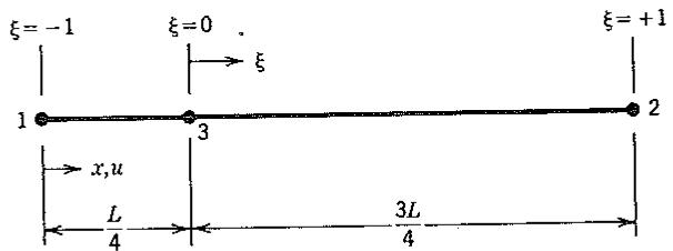
Quarter-Point Elements (QPE). The stress field of Eq. 8.9-1 displays a stress singularity of order $r^{-1/2}$ . An element having side nodes can be made to display a $r^{-1/2}$ stress (or strain) singularity by appropriate definition of its geometry. Consider, for example, the three-node bar element discussed in Section 6.2. This element is shown again in Fig. 8.9-3, now with node 3 moved to the quarter point. With $x_{1}=0$ , $x_{2}=L$ , and $x_{3}=L/4$ , Eq. 6.2-2 yields
text_image
ξ = -1
ξ = 0
ξ = +1
1
3
2
x,u
L
4
3L
4
Figure 8.9-3. Three-node quarter-point bar element.
$^{1}$ Provided that t and a are both at least $2.5(K_{1c}/Y)^{2}$ , where t = specimen thickness and Y = yield strength in a tension test. For smaller values of t and a, fracture toughness is a function of t and a.
$$
x = \frac {L}{4} (1 + \xi) ^ {2} \quad \text { or } \quad \xi = 2 \left(\frac {x}{L}\right) ^ {1 / 2} - 1 \tag {8.9-6}
$$
Equations 6.2-5 and 6.2-7 yield J and $[B]$ , from which $\xi$ may be eliminated by means of Eq. 8.9-6. One obtains
$$
[ \mathbf {B} ] = \left\lfloor \left(\frac {2}{L} - \frac {3}{2 (L x) ^ {1 / 2}}\right), \left(\frac {2}{L} - \frac {1}{2 (L x) ^ {1 / 2}}\right), \left(- \frac {4}{L} + \frac {2}{(L x) ^ {1 / 2}}\right) \right\rfloor \tag {8.9-7}
$$
Accordingly, stress $\sigma_x = E[\mathbf{B}]\{\mathbf{d}\}$ varies as $x^{-1/2}$ —that is, as $r^{-1/2}$ along the line $\theta = 0$ . Stress becomes infinite at $x = 0$ for displacements other than rigid-body motion.
The six-node plane triangle discussed in Section 5.5 can display the $r^{-1/2}$ singularity in its strain field if its side nodes are moved to quarter points near the crack tip, a shown in Fig. 8.9-4 [8.14]. The quarter-point sides should be straight and the side node opposite the crack tip should be at midside.
Another effective singularity element can be formed from a four-sided quadratic element (Fig. 6.6-1a) by collapsing one side to produce a triangle: for example, in Fig. 6.6-1a, nodes 1, 4, and 8 can be assigned the same coordinates and the same displacements. Nodes 5 and 7 are moved to the quarter points near the collapsed side. The side opposite (side 2–6–3 in this example) must be kept straight to avoid significant errors.
Rectangular QPE's—for example, the element of Fig. 6.6-1a with node 1 at the crack tip and nodes 5 and 8 at the quarter points—display the $r^{-1/2}$ singularity only along two sides and the diagonal [8.15]. They are less accurate than triangular QPE's, which display the $r^{-1/2}$ singularity along all rays emanating from the crack tip.
In a QPE, the singularity is precisely at the vertex—that is, at r = 0 in Fig. 8.9-4b. If side nodes are closer to midsides, the singularity moves away from the element (and becomes infinitely distant if side nodes are at midsides). Side nodes need not be precisely at quarter points, as a small error of order e in position produces an error of order $e^{2}$ in the stress intensity factor [8.15]. Indeed, one may
text_image
σ
a
y
x
l
σ
(a)
text_image
y,v
C2
B2
r
x,u
C1
B1
l/4
l
(b)
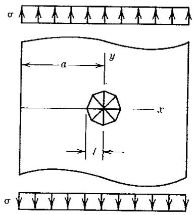
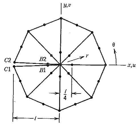
Figure 8.9-4. (a) Plate with edge crack of length a. Only those elements around the crack tip are shown. (b) Mesh of QPE's around the crack tip.
deliberately use an “almost” QPE. In three-dimensional analysis, curvature of the crack front may place the singularity inside a QPE. This trouble may be avoided by placing side nodes a bit closer to midside rather than at quarter points.
In a QPE, strains are represented as a constant plus a term proportional to $r^{-1/2}$ , as may be seen in Eq. 8.9-7. Accordingly, if $\ell / a$ in Fig. 8.9-4 is small, the region of the structure in which the singular stress field is represented decreases. But if $\ell / a$ is large, the nonsingular variations of stress are represented by only the constant term over a larger region of the structure. The best value of $\ell / a$ in a mesh with a fixed number of elements is problem-dependent. Many analyses have used $\ell / a \approx 0.1$ , but the value of $\ell / a$ is not critical in a body of arbitrary geometry if the mesh is adequate to represent stresses in the body were the crack not present [8.16,8.17]. An additional recommendation is that at least four (in a Mode I problem) or eight (in a mixed-mode problem) elements surround the crack tip [8.18]. There is disagreement as to what quadrature rule is best in generating [k] of a QPE.
A common way to calculate stress intensity factors from a finite element analysis is the crack-opening displacement method. From displacements of nodes on $\theta = \pm \pi$ in Fig. 8.9-4 [8.17], it can be shown that QPE's yield the Mode I and Mode II stress intensity factors
$$
K _ {\mathrm{I}} = \frac {2 G}{\kappa + 1} \left(\frac {\pi}{2 \ell}\right) ^ {1 / 2} \left[ \left(4 v _ {B 2} - v _ {C 2}\right) - \left(4 v _ {B 1} - v _ {C 1}\right) \right] \tag {8.9-8a}
$$
$$
K _ {\mathrm{H}} = \frac {2 G}{\kappa + 1} \left(\frac {\pi}{2 \ell}\right) ^ {1 / 2} \left[ \left(4 u _ {B 2} - u _ {C 2}\right) - \left(4 u _ {B 1} - u _ {C 1}\right) \right] \tag {8.9-8b}
$$
where $\kappa$ is given by Eq. 8.9-3.
QPE's have the appeal of simplicity. Elements having side nodes are available in most programs, and they become QPE's when input data locates their side nodes at quarter points. Stress intensity factors are easily computed from Eqs. 8.9-8. However, other methods are available, as follows.
Other Methods. By various methods, including hybrid methods, the strain or stress field used to formulate an element can be made to contain a singularity without invoking special placement of nodes. Indeed, a stress intensity factor can become a d.o.f. in {D}. As alternatives to Eqs. 8.9-8, one can use the virtual crack extension method [8.19] or the J integral.
The simplest alternative is not to use singularity elements at all. Stress intensity factors can be obtained by using ordinary elements to surround the crack tip. Singularity elements merely make possible greater accuracy for a given computational effort.
# 8.10 ELASTIC FOUNDATIONS
Sometimes one elastic structure is supported by another, but stress analysis is required for only the first of the two. Then it suffices to model the effect of the second structure on the first. We need not model the second structure in such detail that stresses within it can be determined. Examples include a rail on a roadbed or a pavement slab on soil. The rail or the slab must be analyzed; the