# 10.5 LOADS WITHOUT AXIAL # SYMMETRY: INTRODUCTION In solids (and shells) of revolution under loads without axial symmetry, we can arrange to compute structural response to each Fourier harmonic of loading from a set of comparatively simple equations that makes no reference to how deformations vary with circumferential coordinate $\theta$ . This set of equations must be solved several times, once for each harmonic of loading. Response attributable to the given loading is found by superposing the separate analyses and, in general, displays deformations that vary with $\theta$ as well as with r and z. The superposition method is much less expensive than a single three-dimensional analysis if only a few Fourier harmonics are needed to represent the load. As examples, wind loading requires few harmonics but a concentrated force requires many. With $\theta$ a principal material direction, the most general stress-strain relation $\{\sigma\} = [\mathbf{E}]\{\epsilon\}$ has the form $$ \left\{ \begin{array}{l} \sigma_ {r} \\ \sigma_ {\theta} \\ \sigma_ {z} \\ \tau_ {z r} \\ \tau_ {r \theta} \\ \tau_ {\theta z} \end{array} \right\} = \left[ \begin{array}{c c c c c c} E _ {1 1} & E _ {1 2} & E _ {1 3} & E _ {1 4} & 0 & 0 \\ & E _ {2 2} & E _ {2 3} & E _ {2 4} & 0 & 0 \\ & & E _ {3 3} & E _ {3 4} & 0 & 0 \\ & & & E _ {4 4} & 0 & 0 \\ \text { symmetric } & & & & E _ {5 5} & E _ {5 6} \\ & & & & & E _ {6 6} \end{array} \right] \left\{ \begin{array}{l} \epsilon_ {r} \\ \epsilon_ {\theta} \\ \epsilon_ {z} \\ \gamma_ {z r} \\ \gamma_ {r \theta} \\ \gamma_ {\theta z} \end{array} \right\} \tag {10.5-1} $$ If $r$ and $z$ are also principal material directions, or if the material is isotropic, then $E_{14} = E_{24} = E_{34} = E_{56} = 0$ . If the material is isotropic, one uses Eq. 10.2-3 and the values $E_{44} = E_{55} = E_{66} = G$ , where $G$ is the shear modulus, $G = 0.5E / (1 + \nu)$ . Let loading of the body be expressed as Fourier series: for example, the radially directed body force is $F_{r} = \Sigma \overline{F}_{rn} \cos n\theta$ , where $\overline{F}_{rn}$ is an amplitude, like $p_{n}$ in Eq. 10.4-1. Thus $$ \left[ \begin{array}{l l l l l} F _ {r} & F _ {z} & \Phi_ {r} & \Phi_ {z} & T \end{array} \right] = \sum_ {n} \left[ \begin{array}{l l l l l} \overrightarrow {F} _ {r n} & \overrightarrow {F} _ {z n} & \overrightarrow {\Phi} _ {r n} & \overrightarrow {\Phi} _ {z n} & \overrightarrow {T} _ {n} \end{array} \right] \cos n \theta \tag {10.5-2a} $$ $$ \left[ \begin{array}{l l} F _ {\theta} & \Phi_ {\theta} \end{array} \right] = \sum_ {n} \left[ \begin{array}{l l} \overline {{F}} _ {\theta n} & \overline {{\Phi}} _ {\theta n} \end{array} \right] \sin n \theta \tag {10.5-2b} $$ where T is temperature, and the $F'$ s and $\Phi$ 's are, respectively, body forces per unit volume and surface tractions in the r, $\theta$ , and z directions. Equations 10.5-2 represent a state of symmetry with respect to the plane $\theta = 0$ (antisymmetric Fourier terms are considered subsequently). We will show that when loads are described by Eqs. 10.5-2, displacements are described by $$ \text { Radial displacement } = u = \sum_ {n} \overline {{u}} _ {n} \cos n \theta \tag {10.5-3a} $$ $$ \text { Circumferential displacement } = v = \sum_ {n} \overline {{v}} _ {n} \sin n \theta \tag {10.5-3b} $$ $$ \text { Axial displacement } = w = \sum_ {n} \overline {{w}} _ {n} \cos n \theta \tag {10.5-3c} $$ All three displacements are needed because the physical problem is three-dimensional. In Eqs. 10.5-2 and 10.5-3, $n$ is an integer, and all barred quantities are functions of $r, z$ , and $n$ but not of $\theta$ . Thus the barred terms are amplitudes. The strain-displacement relations in cylindrical coordinates are $\{\epsilon\} = [\partial]\{\mathbf{u}\}$ ; that is, $$ \left\{ \begin{array}{l} \epsilon_ {r} \\ \epsilon_ {\theta} \\ \epsilon_ {z} \\ \gamma_ {z r} \\ \gamma_ {r \theta} \\ \gamma_ {\theta z} \end{array} \right\} = \left[ \begin{array}{c c c} \partial / \partial r & 0 & 0 \\ 1 / r & \partial / (r \partial \theta) & 0 \\ 0 & 0 & \partial / \partial z \\ \partial / \partial z & 0 & \partial / \partial r \\ \partial / (r \partial \theta) & (\partial / \partial r - 1 / r) & 0 \\ 0 & \partial / \partial z & \partial / (r \partial \theta) \end{array} \right] \left\{ \begin{array}{l} u \\ v \\ w \end{array} \right\} \tag {10.5-4} $$ These relations are independent of material properties and of whether or not $u, v,$ and $w$ are described by series. Consider now a typical single harmonic of displacement, say the nth. If we substitute Eqs. 10.5-3 into Eq. 10.5-4 and the resulting strains into Eq. 10.5-1, we find that stresses of the nth harmonic have the form $$ \left\lfloor \sigma_ {r n} \quad \sigma_ {\theta n} \quad \sigma_ {z n} \quad \tau_ {z r n} \right\rfloor = \left\lfloor \overline {{{\sigma}}} _ {r n} \quad \overline {{{\sigma}}} _ {\theta n} \quad \overline {{{\sigma}}} _ {z n} \quad \overline {{{\tau}}} _ {z r n} \right\rfloor \cos n \theta \tag {10.5-5a} $$ $$ \left[ \tau_ {r \theta n} \quad \tau_ {\theta z n} \right] = \left[ \bar {\tau} _ {r \theta n} \quad \bar {\tau} _ {\theta z n} \right] \sin n \theta \tag {10.5-5b} $$ where the barred quantities are functions of $r$ , $z$ , and $n$ but not of $\theta$ . If Eqs. 10.5-2 and 10.5-5 are substituted into the three differential equations of equilibrium, Eqs. 1.6-4, we find that these three equations assume the forms $$ Q _ {1} \cos n \theta = 0 \quad Q _ {2} \cos n \theta = 0 \quad Q _ {3} \sin n \theta = 0 \tag {10.5-6} $$ where the $Q_{i}$ are functions of r, z, and n but not of $\theta$ . Equations 10.5-6 are analogous to Eq. 10.4-10. Equations 10.5-6 must prevail for all $\theta$ , so $Q_{1} = Q_{2} = Q_{3} = 0$ . As will be seen in Section 10.6, in a finite element context the equations $Q_{1} = Q_{2} = Q_{3} = 0$ produce the equilibrium equations of the nth harmonic $$ [ \mathbf {K} ] _ {n} \{\mathbf {D} \} _ {n} - \{\mathbf {R} \} _ {n} = \{\mathbf {0} \} \tag {10.5-7} $$ Equations 10.5-7 are analogous to Eq. 10.4-11. Their solution yields the nodal d.o.f. $\{\mathbf{D}\}_{n} = [\overline{u}_{1n} - \overline{v}_{1n} - \overline{w}_{1n} - \overline{u}_{2n} \ldots]^T$ , which are displacement amplitudes of the nodal circles in the $n$ th harmonic. Matrix $[\mathbf{K}]_n$ depends on $n$ . The load coefficients in $\{\mathbf{R}\}_{n}$ correspond to the $q_n$ of Eq. 10.4-1. We see that n circumferential waves of loading are associated with n circumferential waves of stress and of displacement. The Fourier harmonics are not coupled. Different numerical values of n present different problems that do not interact. Thus the need for a division into finite elements in the circumferential direction is replaced by the need to superpose separate solutions for a structure divided into finite elements in only its cross section. A single mesh is used for all the separate solutions. In most practical problems only a few load harmonics need be analyzed. A computer program can automatically cycle through a user-specified number of harmonics and superpose the separate solutions. Remarks. The preceding discussion invokes only loads and displacements that have $\theta = 0$ as a plane of symmetry. In general, antisymmetric terms are also present. Thus Eqs. 10.5-2 are augmented to read $$ \left\lfloor F _ {r} \quad F _ {z} \quad \Phi_ {r} \quad \Phi_ {z} \quad T \right] = \sum_ {n} \left\lfloor \overline {{\mathrm{L}}} _ {c n} \right\rfloor \cos n \theta + \sum_ {n} \left\lfloor \overline {{\overline {{\mathrm{L}}}}} _ {s n} \right\rfloor \sin n \theta \tag {10.5-8a} $$ $$ \left[ \begin{array}{l l} F _ {\theta} & \Phi_ {\theta} \end{array} \right] = \sum_ {n} \left[ \overline {{\mathbf {L}}} _ {s n} \right] \sin n \theta + \sum_ {n} \left[ \overline {{\overline {{\mathbf {L}}}}} _ {c n} \right] \cos n \theta \tag {10.5-8b} $$ where $\left\lfloor\overline{L}_{cn}\right\rfloor$ and $\left\lfloor\overline{L}_{sn}\right\rfloor$ represent the symmetric load amplitudes, already present in Eqs. 10.5-2, and $\left\lfloor\overline{L}_{sn}\right\rfloor$ and $\left\lfloor\overline{L}_{cn}\right\rfloor$ represent additional antisymmetric load amplitudes. Similarly, the symmetric displacement field, Eqs. 10.5-3, is augmented by antisymmetric terms and becomes $$ u = \sum_ {n} \bar {u} _ {n} \cos n \theta + \sum_ {n} \bar {\bar {u}} _ {n} \sin n \theta \tag {10.5-9a} $$ $$ v = \sum_ {n} \bar {v} _ {n} \sin n \theta - \sum_ {n} \bar {\bar {v}} _ {n} \cos n \theta \tag {10.5-9b} $$ $$ w = \sum_ {n} \overline {{w}} _ {n} \cos n \theta + \sum_ {n} \overline {{\overline {{w}}}} _ {n} \sin n \theta \tag {10.5-9c} $$ The motivation for the arbitrarily chosen negative sign in the v series is explained in the subsection that follows Eq. 10.6-9. 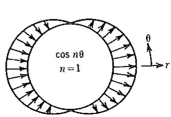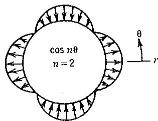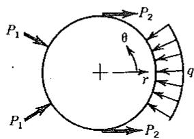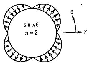Axially symmetric problems are represented by the n = 0 terms of the single-barred series. For $n = 1, 2, 3, \ldots$ , loads and displacements of the single-barred series represent symmetry about the plane $\theta = 0$ . For $n = 0, 2, 4, 6, \ldots$ , loads and deformations have both $\theta = 0$ and $\theta = \pi/2$ as planes of symmetry. Example symmetric loads appear in Fig. 10.5-1c. 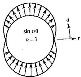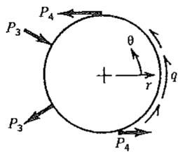Antisymmetric problems (e.g., Fig. 10.5-1f) are represented by the double-barred series. Pure torque is represented by the n = 0 terms of the double-barred series. Thus, for example, we can study the twist of shafts of variable diameter. In the torsion problem u and w are everywhere zero, so a finite element solution based on a stress function is also possible [10.3]. When n = 0, for any node i, nodal d.o.f. $\overline{v}_{ni}$ , $\overline{u}_{ni}$ , and $\overline{w}_{ni}$ have no stiffness associated with them, so these d.o.f. must be suppressed to avoid a singular stiffness matrix. The simplest displacement boundary condition is zero displacement on a nodal circle. This requires that displacement amplitudes on the circle be zero in every harmonic. If loads are symmetric about both the $\theta = 0$ and $\theta = \pi/2$ planes, then u and v are zero at r = 0 in all harmonics. Nonzero and asymmetric displacement conditions can be represented as Fourier series and the separate amplitude coefficients used as prescribed displacements in the separate analyses. Additional constraints on the Fourier displacement amplitudes can be deduced from the condition that strains remain finite at r = 0 [10.4]. If these constraints are not imposed, numerical integration makes some stiffness coefficients significantly larger than others. This circumstance is not likely to be troublesome in static analysis, but it may require a very small time step if explicit integration is applied to transient problems. 

text_image

cos nθ n=1 θ r

(a) 

text_image

cos nθ n = 2 θ r

(b) 

text_image

P₁ P₂ θ r q P₁ P₂

(c) 

text_image

sin nθ n=1 θ r

(d) 

text_image

sin nθ n = 2 θ r

(e) 

text_image

P₄ P₃ θ r q P₃ P₄

(1) Figure 10.5-1. $(a,b)$ Example cosine terms. (c) Possible symmetric loads in an $r\theta$ plane. $(d,e)$ Example sine terms. (f) Possible antisymmetric loads in an $r\theta$ plane. # 10.6 LOADS WITHOUT AXIAL # SYMMETRY: ELEMENT MATRICES Within an element, one can interpolate amplitudes $\overline{u}_{n}$ , $\overline{v}_{n}$ , and $\overline{w}_{n}$ of Eqs. 10.5-3 from nodal amplitudes $\overline{u}_{in}$ , $\overline{v}_{in}$ , and $\overline{w}_{in}$ . Consider, for example, the four-node element in Fig. 10.1-1b. Displacement amplitudes $\{\overline{u}\}_{n}$ in harmonic n are $\{\overline{u}\}_{n} = [\overline{N}]\{\overline{d}\}_{n}$ , in which nodal displacement amplitudes $\{\overline{d}\}_{n}$ pertain to the nth harmonic and are independent of $\theta$ . Written out, this relation is $$ \left\{ \begin{array}{l} \overline {{u}} _ {n} \\ \overline {{v}} _ {n} \\ \overline {{w}} _ {n} \end{array} \right\} = \underbrace {\left[ \begin{array}{c c c} N _ {1} & 0 & 0 \\ 0 & N _ {1} & 0 \\ 0 & 0 & N _ {1} \end{array} \right]} _ {1} \underbrace {\left[ \begin{array}{c c c} N _ {2} & 0 & 0 \\ 0 & N _ {2} & 0 \\ 0 & 0 & N _ {2} \end{array} \right]} _ {2} \underbrace {\left[ \begin{array}{c c c} \dots & \dots & \dots \\ \dots & \dots & \dots \\ \dots & \dots & \dots \\ 3 & 4 \end{array} \right]} _ {4} \{\overline {{\mathbf {d}}} \} _ {n} \tag {10.6-1a} $$ in which element nodal displacement amplitudes are $$ \{\overline {{{\mathbf {d}}}} \} _ {n} = \left[ \begin{array}{l l l l l l l} \overline {{{u}}} _ {1 n} & \overline {{{v}}} _ {1 n} & \overline {{{w}}} _ {1 n} & \overline {{{u}}} _ {2 n} & \overline {{{v}}} _ {2 n} & \overline {{{w}}} _ {2 n} & \dots \end{array} \right] ^ {T} \tag {10.6-1b} $$ For a rectangular four-node element, shape functions $N_{i}$ are as stated in Eq. 10.3-2 (or in Eq. 10.3-4). For an isoparametric four-node element, shape functions $N_{i}$ are as stated in Eqs. 6.3-2. An element with more nodes will display more partitions in Eq. 10.6-1a and more nodal amplitudes in Eq. 10.6-1b. The same shape functions $N_{i}$ can be used for all harmonics. The same interpolation is used for the double-barred series in Eqs. 10.5-9: thus, in Eqs. 10.6-1, single-barred quantities become double-barred quantities. In what follows we discuss the single-barred series. The double-barred series is treated similarly. Summation of the various Fourier harmonics yields displacements in an element is stated by Eqs. 10.5-3. This same displacement field can be written in matrix format by attaching $\cos n\theta$ to rows 1 and 3 in Eq. 10.6-1a and $\sin n\theta$ to row 2, then summing the various harmonics. Thus $$ \left\{ \begin{array}{l} u \\ v \\ w \end{array} \right\} = \sum_ {n} \left\{ \begin{array}{l} \bar {u} _ {n} \cos n \theta \\ \bar {v} _ {n} \sin n \theta \\ \bar {w} _ {n} \cos n \theta \end{array} \right\} = \sum_ {n} \underbrace {\left[ \begin{array}{c c c c} N _ {1} \cos n \theta & 0 & 0 & \dots \\ 0 & N _ {1} \sin n \theta & 0 & \dots \\ 0 & 0 & N _ {1} \cos n \theta & \dots \end{array} \right]} _ {[ \mathrm{N} ] _ {n}} \{\overline {{{\mathbf {d}}}} \} _ {n} \tag {10.6-2} $$ or, with the summation written out, $$ \left\{ \begin{array}{l} u \\ v \\ w \end{array} \right\} = \underbrace {\left[ \begin{array}{l l l l} \mathrm{N} _ {n = 0} & \mathrm{N} _ {n = 1} & \mathrm{N} _ {n = 2} & \dots \end{array} \right] \{\overline {{\mathbf {d}}} \}} _ {[ \mathrm{N} ]} \tag {10.6-3a} $$ in which $\{\overline{\mathbf{d}}\}$ lists amplitudes from all harmonics, that is, $$ \{\overline {{{\mathbf {d}}}} \} = \left\lfloor \{\overline {{{\mathbf {d}}}} \} _ {n = 0} \quad \{\overline {{{\mathbf {d}}}} \} _ {n = 1} \quad \{\overline {{{\mathbf {d}}}} \} _ {n = 2} \quad \dots \right\rfloor^ {T} \tag {10.6-3b} $$ Note that $[N]_{n}$ depends on n only because of the cos $n\theta$ and sin $n\theta$ terms. By applying the operator matrix $[\partial]$ in Eq. 10.5-4, one obtains the strain–displacement relation: $$ \{\epsilon \} = [ \partial ] \left\{ \begin{array}{l} u \\ v \\ w \end{array} \right\} = \underbrace {[ \partial ] \left[ \begin{array}{l l l l} \mathrm{N} _ {n = 0} & \mathrm{N} _ {n = 1} & \mathrm{N} _ {n = 2} & \dots \end{array} \right] \{\overline {{\mathbf {d}}} \}} _ {[ \mathbf {B} ] = [ \mathbf {B} _ {n = 0} \quad \mathbf {B} _ {n = 1} \quad \dots ]} \tag {10.6-4} $$ For example, one determines that the contribution of the $n$ th harmonic to strains, $\{\pmb{\epsilon}\}_{n} = [\mathbf{B}]_{n}\{\mathbf{d}\}_{n}$ , is $$ \left\{ \begin{array}{l} \epsilon_ {r n} \\ \epsilon_ {\theta n} \\ \epsilon_ {z n} \\ \gamma_ {z r n} \\ \gamma_ {r \theta n} \\ \gamma_ {\theta z n} \end{array} \right\} = \underbrace {\left[ \begin{array}{c c c c} N _ {1 , r} \cos n \theta & 0 & 0 & \dots \\ \frac {N _ {1}}{r} \cos n \theta & \frac {n N _ {1}}{r} \cos n \theta & 0 & \dots \\ 0 & 0 & N _ {1 , z} \cos n \theta & \dots \\ N _ {1 , z} \cos n \theta & 0 & N _ {1 , r} \cos n \theta & \dots \\ - \frac {n N _ {1}}{r} \sin n \theta & \left(N _ {1 , r} - \frac {N _ {1}}{r}\right) \sin n \theta & 0 & \dots \\ 0 & N _ {1 , z} \sin n \theta & - \frac {n N _ {1}}{r} \sin n \theta & \dots \end{array} \right]} _ {1} \underbrace {\left\{ \begin{array}{l} \bar {u} _ {1 n} \\ \bar {v} _ {1 n} \\ \bar {w} _ {1 n} \\ \vdots \end{array} \right\}} _ {2, 3, 4,..} \tag {10.6-5} $$ where the partitioning corresponds to that used in Eq. 10.6-1a. If the element is isoparametric, the usual transformation of derivatives must be included (see e.g. Eq. 6.3-7): $$ N _ {i, r} = \Gamma_ {1 1} N _ {i, \xi} + \Gamma_ {1 2} N _ {i, \eta} \quad \text { and } \quad N _ {i, z} = \Gamma_ {2 1} N _ {i, \xi} + \Gamma_ {2 2} N _ {i, \eta} \tag {10.6-6} $$ Shape functions $N_{i}$ depend on r and z. Therefore, we see from Eq. 10.6-5 that [B] is a function of r, z, n, and $\theta$ . The element stiffness matrix is given by Eq. 10.3-3 or Eq. 10.3-7. Let there be J nodes per element and M harmonics included in the summation. Then the integrand matrix $[B]^{T}[E][B]$ is a full matrix of size 3JM by 3JM. It is composed of an M by M array of 3J by 3J submatrices. The off-diagonal submatrices contain $\sin m\theta$ sin $n\theta$ or $\cos m\theta$ cos $n\theta$ in every term, where m and n are different integers. According to Eqs. 10.4-2, these terms integrate to zero. We are left with only M on-diagonal submatrices, each 3J by 3J and containing $\sin^{2} n\theta$ or $\cos^{2} n\theta$ in every term. After integration according to Eqs. 10.4-2, the common factor $\pi$ (or $2\pi$ for n = 0) appears in every term. Integration with respect to r and z (or $\xi$ and $\eta$ ) is done as though the problem were axially symmetric. After integration is complete, terms in each 3J by 3J submatrix have the form $A + Bn^{2}$ or the form Cn, where A, B, and C depend on material properties and element geometry but are independent of n and $\theta$ . Accordingly, the various expressions here symbolized by A, B, and C need be generated only once, regardless of the number of harmonics used. Element equations, and structural equations after assembly of elements, have the respective forms $$ \left[ \begin{array}{c c c c} \mathbf {k} _ {0} & & & \\ & \mathbf {k} _ {1} & & \\ & & \ddots & \\ & & & \ddots \end{array} \right] \left\{ \begin{array}{l} \overline {{\mathbf {d}}} _ {0} \\ \overline {{\mathbf {d}}} _ {1} \\ \cdot \\ \cdot \\ \cdot \end{array} \right\} = \left\{ \begin{array}{l} \overline {{\mathbf {r}}} _ {0} \\ \overline {{\mathbf {r}}} _ {1} \\ \cdot \\ \cdot \\ \cdot \end{array} \right\} \quad \text {and} \quad \left[ \begin{array}{c c c c} \mathbf {K} _ {0} & & & \\ & \mathbf {K} _ {1} & & \\ & & \ddots & \\ & & & \ddots \end{array} \right] \left\{ \begin{array}{l} \overline {{\mathbf {D}}} _ {0} \\ \overline {{\mathbf {D}}} _ {1} \\ \cdot \\ \cdot \\ \cdot \end{array} \right\} = \left\{ \begin{array}{l} \overline {{\mathbf {R}}} _ {0} \\ \overline {{\mathbf {R}}} _ {1} \\ \cdot \\ \cdot \\ \cdot \end{array} \right\} \tag {10.6-7} $$ where each $[k]_{n}$ is of size 3J by 3J, and subscripts 0, 1, and so on indicate the number of the Fourier harmonic. The M separate harmonics are not coupled. In practice, matrices are not built for all harmonics at once (as Eqs. 10.6-7 seem to imply). Instead, as suggested by Eq. 10.5-7, separate harmonics of loading are analyzed serially, with results stored for subsequent superposition. Element loads (Eq. 4.1-6) include contributions such as $$ \{\mathbf {r} \} = \int_ {V _ {e}} [ \mathbf {N} ] _ {3 J M \times 3} ^ {T} \left\{\mathbf {F} \right\} d V + \int_ {V _ {e}} [ \mathbf {B} ] _ {3 J M \times 6} ^ {T} \left[ \mathbf {E} \right] _ {6 \times 6} \left\{\boldsymbol {\epsilon} _ {0} \right\} d V \tag {10.6-8} $$ where [N] and [B] are given by Eqs. 10.6-3a and 10.6-4. Body forces {F} are, from Eq. 10.5-8, $$ \{\mathbf {F} \} = \left\{ \begin{array}{l} \overline {{{F}}} _ {r 0} + \overline {{{F}}} _ {r 1} \cos \theta + \overline {{{F}}} _ {r 2} \cos 2 \theta + \dots \\ 0 + \overline {{{F}}} _ {\theta 1} \sin \theta + \overline {{{F}}} _ {\theta 2} \sin 2 \theta + \dots \\ \overline {{{F}}} _ {z 0} + \overline {{{F}}} _ {z 1} \cos \theta + \overline {{{F}}} _ {z 2} \cos 2 \theta + \dots \end{array} \right\} \tag {10.6-9} $$ Initial strains $\{\epsilon_{0}\}$ are written similarly. Integration of Eq. 10.6-8 according to Eqs. 10.4-2 shows that $\{\bar{r}\}_{0}$ in Eq. 10.6-7 contains only the zero-harmonic (axially symmetric) load terms, $\{\bar{r}\}_{1}$ contains only the first-harmonic load terms, and so on. Thus again we see the uncoupling of harmonics. In the pure torsion harmonic n = 0, nodal d.o.f. $\overline{u}_{ni}$ and $\overline{w}_{ni}$ have no stiffness associated with them. In the axially symmetric harmonic n = 0, nodal d.o.f. $\overline{v}_{ni}$ have no stiffness associated with them. These d.o.f. must be suppressed in Eqs. 10.6-7. Stresses in an element are computed in the usual way, that is, by the equation $\{\sigma\} = [E]([B]\{d\} - \{\epsilon_{0}\})$ , in which [B] is as stated in Eq. 10.6-4. Thus stresses from the various harmonics are superposed. Antisymmetric Harmonics. When the double-barred terms in Eqs. 10.5-8 and 10.5-9 are used, the preceding arguments are almost unchanged. One finds that $\sin n\theta$ and $\cos n\theta$ are interchanged in Eqs. 10.6-2, 10.6-5, and 10.6-9. In addition, algebraic signs change in the last two rows of $[\mathbf{B}]_n$ in Eq. 10.6-5. However, one finds that stiffness matrices $[\mathbf{k}]_0$ , $[\mathbf{k}]_1$ , and so on, in Eq. 10.6-7 are identical to those obtained in the symmetric case. This convenience is the motivation for the arbitrarily chosen negative sign in Eqs. 10.5-9: if the sign were positive instead, the $[\mathbf{k}]_i$ for a given $i$ would differ between symmetric and antisymmetric cases. More General Elastic Properties. If $\theta$ is not a principal material direction, [E] in Eq. 10.5-1 becomes a full matrix, and each stress in Eq. 10.5-5 depends on both $\sin n\theta$ and $\cos n\theta$ . Symmetric and antisymmetric terms are now coupled in each harmonic, but different harmonics are uncoupled. Thus Eqs. 10.6-7 are still valid, but each $[\mathbf{k}]_n$ is now $6J$ by $6J$ in size. Details of these arguments appear in [10.5]. The problem is more difficult if elastic properties depend on $\theta$ . One physical cause of this circumstance is the combination of temperature-dependent moduli and a $\theta$ -dependent temperature field. A Fourier series attack can again be used, but all harmonics are coupled [10.6,10.7]. # 10.7 RELATED PROBLEMS The Fourier series treatment described in Sections 10.5 and 10.6 is also known as the semianalytical method and the separation of variables method. When used for plates, it is called the finite strip method. Besides its application to plates and to solids and shells of revolution, the Fourier series method can be applied to prismatic solids [10.8,10.9]. Then the name finite prism method may be used. The solid, and its elements, are prismatic (Fig. 10.7-1). The displacement field is again Eq. 10.5-9, except that $\pi y/L$ replaces $\theta$ . If only the single-barred series are used, deformation and loading are symmetric about the xz plane, with v = 0 at y = 0 and at $y = \pm L$ . As usual, arbitrary loads and displacements are treated by determining their Fourier coefficients and making a separate analysis for each, then superposing results. Problems such as that of Fig. 10.7-1 may require 9 to 19 Fourier coefficients. In a physical sense, what has been done in Fig. 10.7-1 is to take a toroidal solid that extends from $-\pi$ to $\pi$ and straighten it out to form a prismatic solid that extends from -L to L. 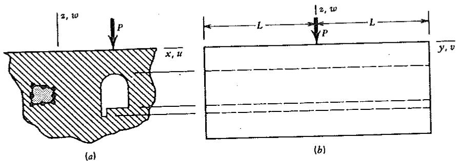The straightening can be “faked” by moving the z axis  Figure 10.7-1. A point load P over a long tunnel. A suitably large portion of the surrounding earth or rock is modeled by finite elements, one of which is shown and shaded. (a) Front view. (b) Right-side view. in Fig. 10.7-1a far to the left and making it an axis of revolution. Then the almost-prismatic solid can be analyzed by a computer program for solids of revolution. The problem of a curved beam bent by a moment $M_0$ is axially symmetric in geometry and material properties. But it is not obvious that an axisymmetric analysis can deal with a moment loading. Reference 10.10 describes how. The trick is to use a thermal load to simulate the strains produced by $M_0$ . Note that if the curved beam is a thin-walled pipe elbow, its cross section becomes oval in response to $M_0$ and therefore is more flexible than a pipe whose cross section remains circular. Pipe elbow elements that include this effect have been developed [10.11]. Some geometries are “almost” axially symmetric, for example, the geometry or material properties have modest departures from $\theta$ independence, or an axially symmetric body is attached to a body that has no symmetry. Aspects of such problems are discussed in [10.7,10.12,10.13]. # PROBLEMS # Section 10.2 10.1 If a problem is to be mathematically two-dimensional, $\theta$ independence is required of all dependent variables. Explain by example why this requires that $\theta$ be a principal direction of an orthotropic material. Suggestion: Consider axial load on a cylinder. # Section 10.3 10.2 Imagine that Fig. 6.12-1 depicts displacements and deformations of the square cross section of an axially symmetric four-node element. The axis of revolution is to the left of each cross section. For parts (a) and (b), identify each of the eight modes: that is, is it a rigid-body mode, a zero-energy deformation mode, or a straining mode? (a) Let [k] be generated by one-point Gauss quadrature. (b) Let [k] be generated by four-point Gauss quadrature. 10.3 Arguments are presented in Section 6.11 regarding the number of Gauss points needed for correct volume calculation and correct convergence of computed results. Reference there is to plane elements. How should these arguments be amended if reference is to axially symmetric elements instead? 10.4 Revise Figs. 6.5-1 and 6.5-2 to deal with an axially symmetric problem; that is, describe precisely what changes and additions are necessary. 10.5 Consider an axially symmetric element whose cross section is a three-node triangle. The displacement field has the form seen in Eq. 4.2-9. Determine stiffness matrix $[k_{a}]$ , which is defined by Eq. 4.1-18, to the extent of writing the integrand in detail and computing the product $[B_{a}]^{T}[E][B_{a}]$ . Use [E] from Eq. 10.2-2. 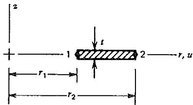10.6 The sketch shows the cross section of a flat element shaped like a metal washer. D.o.f. are radial displacements $u_{1}$ and $u_{2}$ at nodal circles 1 and 2. The material is isotropic. (a) Formulate matrices [N] and [B]. (b) Let $\nu = 0$ , and generate [k] for a one-radian segment by explicit integration. (c) Let $L = r_2 - r_1$ and $r_m = (r_1 + r_2)/2$ . Simplify integration by assuming that $r = r_m$ . Hence, determine [k] (for a nonzero Poisson's ratio). For what geometry is this [k] a good approximation? (d) For $\nu = 0$ , show that the [k]'s of parts (b) and (c) agree for $r_m >> L$ . (e) From part (b), obtain [k] for the special case $\nu = r_1 = u_1 = 0$ . (f) From part (c), obtain [k] for the special case $\nu = r_1 = u_1 = 0$ . 

text_image

z 1 t 2 r, u r₁ r₂

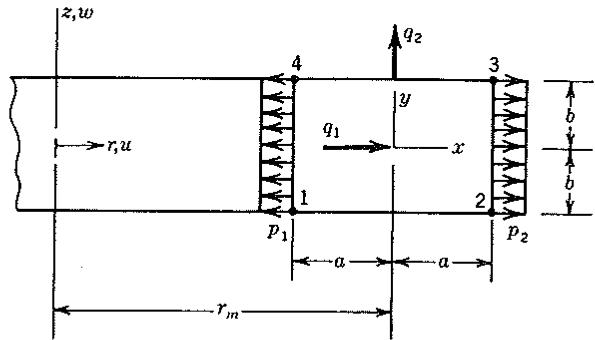
Problem 10.6 10.7 The four-node axisymmetric element shown has a rectangular cross section of dimensions $2a$ and $2b$ . The material is homogeneous, isotropic, and has mass density $\rho$ . Evaluate element nodal loads $\{\mathbf{r}_e\}$ produced by the following actions. (a) Uniform radial pressure $p_1$ (tensile). (b) Uniform radial pressure $p_{2}$ (tensile). (c) Line load $q_{1}$ (units N/m), which acts at $x = y = 0$ . (d) Line load $q_{2}$ (units N/m), which acts at $x = 0$ , $y = b$ . 

text_image

z,w 4 q2 3 y q1 x 1 2 p1 a a p2 r,u b b rm

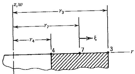
Problem 10.7 (e) Uniform heating an amount $T$ . Stop after setting up a triple integral over $d\theta dx dy$ . (f) Rotation at constant angular velocity $\omega$ . Stop after setting up a triple integral over $d\theta dx dy$ . 10.8 The sketch represents three nodes on a $z =$ constant face of an axisymmetric quadratic element. Node 7 is at midside. Determine the consistent nodal load vector for these three nodes if $z$ -direction surface traction $\Phi_z$ is applied as follows. (a) $\Phi_{z}$ is the constant value $p$ over the face. (a) $\Phi_z$ is the constant value $p_1$ with $\Phi_z = (\xi^2 - \xi)p_4/2 + (1 - \xi^2)p_7 + (\xi^2 + \xi)p_3/2$ , which is a parabolic variation based on nodal values $p_4, p_7$ , and $p_3$ . 

text_image

z₁w r₃ r₇ r₄ 4 7 3 r ξ

Problem 10.8 10.9 In the sketch for Problem 10.8, imagine that $r_4 = 0$ , and that $w_4 > 0$ and $w_7 = w_3 = 0$ . Is such a deformation mode reasonable? What do you conclude about $\gamma_{zr}$ at $r = 0$ ? 10.10 Show that $\epsilon_r = \epsilon_\theta$ at $r = 0$ in an axially symmetric problem. # Section 10.4 10.11 (a) Use Eqs. 10.4-2 to verify the right-hand sides of Eqs. 10.4-3. (b) Verify the expression for $q_{n}$ in Eq. 10.4-4. (b) Verify the expression for $q_{n}$ is given by (c) Verify the expression for $q_{n}$ in Eq. 10.4-5. Suggestion: Imagine that $P$ is generated by a distributed load of large intensity acting over a small length. (d) Determine a Fourier series that represents two radial loads $P$ on a disk, one outward at $\theta = -\pi / 2$ and another outward at $\theta = +\pi / 2$ . 10.12 Use Eqs. 10.4-12 to compute the center deflection and center bending moment in a uniform simply supported beam. Use one, then two, then three series terms, each time computing the percentage error of the approximation. (a) Consider a uniformly distributed upward load. (b) Consider a concentrated downward load at midspan. 10.13 A uniform, simply supported beam is loaded by a linearly varying distributed load that has intensity $q_{L}$ at $x = L$ , as shown. (a) Determine a Fourier series representation of the load. (a) Determine a Fourier series of $x = L/2$ , hence, determine the deflection and the bending moment at x = L/2, using 1, 2, and 3 series terms. Compute the percentage error of each of these approximations.