Combination of Eqs. 12.5-7, 12.5-8, and 12.5-9 yields $$ \left[ \begin{array}{l l l l l l} \epsilon_ {x} & \epsilon_ {y} & \epsilon_ {z} & \gamma_ {x y} & \gamma_ {y z} & \gamma_ {z x} \end{array} \right] ^ {T} = \sum \left[ \mathbf {B} _ {i} \right] \left[ \begin{array}{l l l l l} u _ {i} & v _ {i} & w _ {i} & \alpha_ {i} & \beta_ {i} \end{array} \right] ^ {T} \tag {12.5-10} $$ The complete strain-displacement matrix [B] is built of as many 6 by 5 blocks $[\mathbf{B}_i]$ as there are nodes in the element. Stiffness Matrix [k]. The stress–strain relation can be stated as $$ \{\boldsymbol {\sigma} \} = [ \mathrm{E} ] \{\boldsymbol {\epsilon} \} \quad \text { or as } \quad \{\boldsymbol {\sigma} ^ {\prime} \} = [ \mathrm{E} ^ {\prime} ] \{\boldsymbol {\epsilon} ^ {\prime} \} \tag {12.5-11} $$ where $\{\sigma\}$ contains stresses in Cartesian directions xyz and $\{\sigma'\}$ contains stresses in local directions normal and tangent to the shell midsurface. The latter relation is $^{2}$ $$ \left\{ \begin{array}{l} \sigma_ {1} \\ \sigma_ {2} \\ \sigma_ {3} \\ \tau_ {1 2} \\ \tau_ {2 3} \\ \tau_ {3 1} \end{array} \right\} = \underbrace {\left[ \begin{array}{c c c c c c} E _ {1 1} & E _ {1 2} & 0 & 0 & 0 & 0 \\ E _ {1 2} & E _ {2 2} & 0 & 0 & 0 & 0 \\ 0 & 0 & 0 & 0 & 0 & 0 \\ 0 & 0 & 0 & G _ {1 2} & 0 & 0 \\ 0 & 0 & 0 & 0 & 5 G _ {2 3} / 6 & 0 \\ 0 & 0 & 0 & 0 & 0 & 5 G _ {3 1} / 6 \end{array} \right]} _ {[ \mathbf {E} ^ {\prime} ]} \left\{ \begin{array}{l} \epsilon_ {1} \\ \epsilon_ {2} \\ \epsilon_ {3} \\ \gamma_ {1 2} \\ \gamma_ {2 3} \\ \gamma_ {3 1} \end{array} \right\} \tag {12.5-12} $$ where directions 1 and 2 are tangent to the midsurface and direction 3 is normal to it. These directions are presumed to be principal material directions if the material is orthotropic. The factors of 5/6 account for a parabolic variation of transverse shear strain through the thickness. Note that Eq. 12.5-12 is contrived to make the transverse normal stress $\sigma_{3}$ equal to zero. [E] is obtained from $[E']$ by the coordinate transformation $[E] = [T_{\epsilon}]^{T}[E'][T_{\epsilon}]$ (see Eq. 7.3-10). This transformation must be carried out at each Gauss point used in generating [k] by numerical integration. Direction cosines needed in $[T_{\epsilon}]$ are the direction cosines of vectors $V_{1}$ , $V_{2}$ , and $V_{3}$ at the Gauss point. In turn, these vectors can be found by shape function interpolation from nodal values, $$ \mathbf {V} _ {1} = \sum N _ {i} \mathbf {V} _ {1 i} \quad \mathbf {V} _ {2} \doteq \sum N _ {i} \mathbf {V} _ {2 i} \quad \mathbf {V} _ {3} = \sum N _ {i} \mathbf {V} _ {3 i} \tag {12.5-13} $$ in which the $N_{i}$ are evaluated at the Gauss point in question. The element stiffness matrix is $$ \underset {5 N \times 5 N} {[ \mathbf {k} ]} = \int_ {- 1} ^ {1} \int_ {- 1} ^ {1} \int_ {- 1} ^ {1} \underset {5 N \times 6} {[ \mathbf {B} ] ^ {T}} \underset {6 \times 6} {[ \mathbf {E} ]} \underset {6 \times 5 N} {[ \mathbf {B} ]} \det [ \mathbf {J} ] d \xi d \eta d \zeta \tag {12.5-14} $$ where N is the number of nodes per element. If material properties are independent of $\zeta$ , and if small errors are acceptable [12.7], then thickness-direction integration can be done explicitly. In doing so one discards terms in [J] that depend on $\zeta$ , under the assumption that these terms are negligible if the element is not sharply curved. Next, [B] is split into a part $[B_{0}]$ that is independent of $\zeta$ and a part $\zeta[B_{1}]$ that is linear in $\zeta$ , so that $[B] = [B_{0}] + \zeta[B_{1}]$ . Thus terms linear in $\zeta$ integrate to zero and Eq. 12.5-14 becomes $$ [ \mathbf {k} ] = \int_ {- 1} ^ {1} \int_ {- 1} ^ {1} (2 [ \mathbf {B} _ {0} ] ^ {T} [ \mathbf {E} ] [ \mathbf {B} _ {0} ] + \frac {2}{3} [ \mathbf {B} _ {1} ] ^ {T} [ \mathbf {E} ] [ \mathbf {B} _ {1} ]) \det [ \mathbf {J} ] d \xi d \eta \tag {12.5-15} $$ in which [J] remains 3 by 3 but is evaluated on the midsurface, $\zeta = 0$ . Difficulties arising from shear locking, membrane locking, and mechanisms can be dealt with by selective and reduced integration and other strategies $[12.13]$ . As an element becomes thin, the penalty matrix associated with transverse shear must not be allowed to overwhelm the rest of the stiffness matrix (see the remarks that close Section 9.4). Element nodal loads (Eq. 4.1-6) come from the usual sources. Those associated with initial strains are, since $\{\epsilon_{0}^{\prime}\} = [T_{\epsilon}]\{\epsilon_{0}\}$ , $$ \int_ {V _ {\epsilon}} [ \mathbf {B} ] ^ {T} [ \mathbf {E} ] \{\boldsymbol {\epsilon} _ {0} \} d V = \int_ {- 1} ^ {1} \int_ {- 1} ^ {1} \int_ {- 1} ^ {1} [ \mathbf {B} ] ^ {T} [ \mathbf {T} _ {\epsilon} ] ^ {T} [ \mathbf {E} ^ {\prime} ] \{\boldsymbol {\epsilon} _ {0} ^ {\prime} \} \det [ \mathbf {J} ] d \xi d \eta d \zeta \tag {12.5-16} $$ Finally, element stresses referred to local directions 1–2–3 are $$ \{\sigma^ {\prime} \} = [ \mathrm{E} ^ {\prime} ] ([ \mathrm{T} _ {\epsilon} ] [ \mathrm{B} ] \{\mathrm{d} \} - \{\epsilon_ {0} ^ {\prime} \}) \tag {12.5-17} $$ Stresses at Gauss points may be more accurate than stresses computed elsewhere in the element, as noted in Section 6.13. Usually, elements share a common tangent plane at each interelement boundary. Thus d.o.f. $\alpha_{i}$ and $\beta_{i}$ are midsurface-tangent vectors in all elements that share node i. This ideal circumstance would disappear if elements were to form a ridge line where they meet, as in a folded plate. Then $V_{3i}$ could be defined as an average shell normal vector, with $\alpha_{i}$ and $\beta_{i}$ normal to $V_{3i}$ , but accuracy loss would be expected. # PROBLEMS # Section 12.1 12.1 In terms of $R_{s}$ and $R_{\theta}$ , how would you qualitatively describe the shape of an American football? 12.2 According to elementary stress formulas and Eqs. 12.1-1, what are $N_x$ , $N_y$ , and $N_{xy}$ for a cylindrical tank under internal pressure? 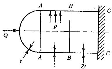12.3 The cylindrical tank shown contains a step change in thickness and is capped by a hemispherical shell. Loads consist of axial force $Q$ and internal pressure $p$ . (a) Explain why load Q cannot be supported by membrane action only. (b) Free the built-in support condition at CC and divide the vessel into three parts by making circumferential cuts along AA and BB. Then show by a sketch the displaced shape of each part produced by pressure p alone. (c) Show by a sketch the loads (applied by one part to another) needed to restore continuity of displacements. 

text_image

A B C p Q t A B C t 2t

Problem 12.3 12.4 Imagine that a garden hose has an elliptical cross section. Explain why internal pressure causes bending stresses to appear, and sketch their approximate variation over the outside perimeter of the cross section. Also explain why, if internal pressure is to be carried by membrane stresses alone, the cross section must first become circular. # Section 12.2 12.5 Write an expression for strain $\epsilon_s$ if the arch radius $R$ is a function of $s$ . 12.6 (a) Derive Eqs. 12.2-4. Suggestion: Combine Eqs. 12.2-2 and integrate the resulting differential equation. (b) Consider a quarter-circle arch that occupies the first quadrant of a Cartesian reference frame. By three separate sketches, show the displacement fields associated with $b_{1}, b_{2}$ , and $b_{3}$ in Eqs. 12.2-4. 12.7 Write the coordinate transformation of nodal d.o.f. for a straight element; that is, define all terms completely in terms of $L$ and $R$ . Assume that local d.o.f. are ordered as shown in Eq. 12.2-6, and that global d.o.f. in Fig. 12.2-3b have the order $\left[ D_{s1} \quad D_{r1} \quad \beta_1 \quad D_{s2} \quad D_{r2} \quad \beta_2 \right]^T$ . 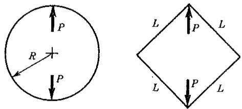12.8 Model a complete circular ring by four straight elements of equal length. The model is therefore a square, as shown. Compute the relative separation of loads $P$ , accounting for bending stiffness only. Take the element length as (a) chord length $L = \sqrt{2} R$ , and (b) arc length $L = \pi R / 2$ . 

text_image

P R P L P L P L

Problem 12.8 12.9 For a curved arch, integrate $U_{m}$ of Eq. 12.2-3 using the displacement field of Eqs. 12.2-7. Hence, show that the condition $U_{m} = 0$ implies Eqs. 12.2-9. 12.10 Using the following displacement fields for a curved arch, establish the relation between nodal d.o.f. and the $a_{i}$ ; that is, find [A] in the relation $$ \left\lfloor u _ {1} \quad w _ {1} \quad \beta_ {1} \quad u _ {2} \quad w _ {2} \quad \beta_ {2} \right\rfloor^ {T} = [ \mathrm{A} ] \left\lfloor a _ {1} \quad a _ {2} \quad a _ {3} \quad a _ {4} \quad a _ {5} \quad a _ {6} \right\rfloor^ {T} $$ where $\beta = w_{,s}$ . (a) Use Eqs. 12.2-7. (b) Use Eqs. 12.2-11. 12.11 Would the mode associated with d.o.f. $a_7$ in Eq. 12.2-12a be of any benefit to (a) the straight element of Fig. 12.2-3a, or (b) the curved element based on Eqs. 12.2-7? Consider both full and selective integration in your explanation of part (b). 12.12 In the stiffness matrix of the element associated with Eqs. 12.2-11, the diagonal coefficients associated with nodal deflections $w_{1}$ and $w_{2}$ are each $$ k = \frac {E I}{R ^ {3}} \left(\frac {2 4}{\lambda^ {3}} - \frac {1 9 2}{3 5 \lambda} + \frac {1 6 \lambda}{3 5}\right) $$ where $\lambda = L / 2R$ for an element of arc length $L$ . Use this information to solve for the deflection of load $P$ in Fig. 12.2-1a from a two-element model. 12.13 In formulating an element stiffness matrix [k] from Eqs. 12.2-11, energy $U_{m}$ makes no contribution to [k]. Why cannot $U_{m}$ simply be discarded in formulating other curved arch elements, for example, those associated with Eqs. 12.2-7 and 12.2-13? 12.14 (a) Verify Eqs. 12.2-17 and 12.2-18. (b) Determine the analogous equations of constraint that pertain to use of reduced integration for $U_{m}$ and $U_{s}$ . 12.15 Investigate the $\gamma_{zs} = 0$ condition and the effect of reduced integration on the three-node Mindlin element (analogous to Eqs. 12.2-20 and 12.2-21). # Section 12.3 12.16 Consider a doubly curved shell, modeled by flat triangular elements, such as those of Eqs. 12.3-2 and 12.3-3. What can you say about interelement compatibility of edge displacements? 12.17 Write an equation analogous to Eq. 12.3-4 but appropriate to a flat element that has four nodes. Do you think this equation should be used if the element is warped rather than flat? 12.18 Imagine that each side of a rectangular box is modeled by a mesh of flat shell elements. Internal pressure is applied. Along the edges where sides intersect, what d.o.f. can probably be set to zero, and why? # Section 12.4 12.19 (a) Derive Eqs. 12.4-2. (b) Rewrite Eqs. 12.4-2 in a form appropriate to a shell with a straight meridian. 

text_image

T r₁ s L t φ

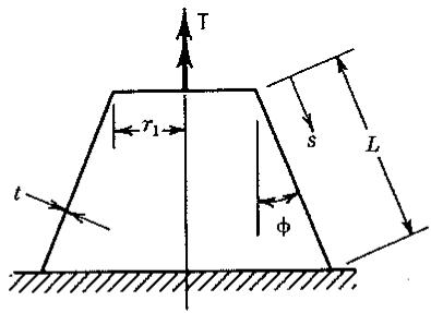
Problem 12.20 12.20 The conical shell shown is fixed at its base and loaded by torque T at the top. Use mechanics of materials concepts, not finite elements, to answer the following questions. (a) What is shear stress $\tau_{s\theta}$ , in terms of $T$ , $r_1$ , $t$ , $\phi$ , and $s$ ? (b) What is the angle of rotation of the top of the truncated cone relative to the bottom, in terms of $T$ , $r_1$ , $t$ , $\phi$ , $L$ , and shear modulus $G$ ? 12.21 Specialize Eqs. 12.4-4 to the following cases. (a) A cylindrical shell, with $s$ the only independent variable. (b) A flat plate, with $r$ the only independent variable. (c) A sphere, with $\phi$ the only independent variable. 12.22 Consider a thin cylindrical shell of radius R whose midsurface axial strain $\epsilon_{m}$ is unrestrained. By considering the energy associated with membrane strains $\epsilon_{ms}$ and $\epsilon_{m\theta}$ , show that displacement w is in effect resisted by an elastic foundation of modulus $Et/R^{2}$ (as well as being resisted by bending stiffness). 12.23 Consider a cylindrical shell, thin-walled and symmetrically loaded, but without axial loads. Thus $N_{s} = 0$ , $\epsilon_{ms} = -\nu\epsilon_{m\theta}$ , and displacement u need not be considered. Generate the 4 by 4 element stiffness matrix. Use a cubic w field. 12.24 Show that $\gamma_{zs}$ at $s = 0$ from Eq. 12.4-10 is the same as $\gamma_{zs}$ for all $s$ from Eq. 12.4-13. 12.25 Show that application of Eq. 12.4-12 converts Eqs. 12.4-10 and 12.4-11 to Eqs. 12.4-13 and 12.4-14. 12.26 Verify the remark made in the sentence following Eq. 12.4-14. 12.27 Let a constant pressure p be applied to the inside surface of the element described by Eq. 12.4-13. Evaluate the consistent element nodal load vector. 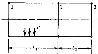12.28 The cylindrical shell shown is modeled by two Mindlin elements, prevented from rotation $\beta$ at nodal circles 1 and 3, and loaded by a uniform radial pressure on the inside surface. There are no end caps. Consistently computed nodal loads are applied. Will computed results display nonzero meridional curvature $\kappa_{s}$ in the following situations? Answer without doing calculations. (a) $L_{1} = L_{2}$ , and $w$ varies linearly between nodes. (b) $L_{1} \neq L_{2}$ , and $w$ varies linearly between nodes. (c) $L_{1} = L_{2}$ , and the element of Eqs. 12.4-13 is used. (d) $L_{1} \neq L_{2}$ , and the element of Eqs. 12.4-13 is used. 

text_image

1 2 3 L₁ L₂

Problem 12.28 # Section 12.5 12.29 Write an equation analogous to Eq. 12.5-2 but applicable to the element of Fig. 12.5-1b. (Each shape function should depend on $\xi$ and $\eta$ and should be multiplied by a linear function of $\zeta$ .) 12.30 (a) Define terms in the Jacobian matrix [J] in terms of $\zeta$ , $N_{i}$ , $N_{i,\xi}$ , $N_{i,\eta}$ , nodal coordinates, and components of $\mathbf{V}_{3i}$ . (b) Specialize your result for the case of an element that is flat, of constant thickness, and whose midsurface coincides with the xy plane. 12.31 (a) Imagine that instead of rotational d.o.f. $\alpha_{i}$ and $\beta_{i}$ in Fig. 12.5-2, we elect to use rotational d.o.f. $\beta_{xi}$ , $\beta_{yi}$ , and $\beta_{zi}$ , which are small rotations about axes $x$ , $y$ , and $z$ . Write the appropriate form of Eq. 12.5-6 and define the terms in the direction cosine matrix $[\mu_i]$ you use. (b) Check that your formula agrees with Eq. 12.5-6 for the special cases of all vectors $\mathbf{V}_3$ parallel to the $x$ axis, then the $y$ axis, and finally the $z$ axis. (c) The element now has six d.o.f. per node rather than five. What possible difficulty does this element present? 12.32 (a) How can the transformation of $[\mathbf{E}']$ to $[\mathbf{E}]$ be made more computationally efficient? (Exploit the null row and the null column in $[\mathbf{E}']$ .) (b) Write Eq. 12.5-14 in a form that uses $[E']$ rather than $[E]$ . 12.33 Let a typical $[B_{i}]$ in Eq. 12.5-10 have the form $[B_{i}] = [H][\overline{B}_{i}]$ , where $[H]$ is defined by Eq. 6.7-5 and $[\overline{B}_{i}]$ is a 9 by 5 matrix. Express $[\overline{B}_{i}]$ as a function of $\zeta$ , $t_{i}$ , $N_{i}$ , $N_{i,\xi}$ , $N_{i,\eta}$ , direction cosines, and the $\Gamma_{ij}$ in $[\Gamma] = [J]^{-1}$ . 12.34 Two elements of the type shown by Fig. 12.5-1c are to be connected side by side. However, they do not share a common tangent plane; for example, they may be perpendicular, like adjacent sides of a box. How should the connection be accomplished?—that is, how should d.o.f. along the connection line be treated? 12.35 Consider a membrane shell (a shell that has no bending stiffness). Review the formulations presented in Section 12.5, and state how they may be simplified or specialized to deal with a membrane shell. 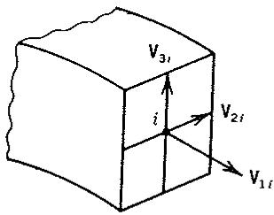12.36 The sketch represents an end of an isoparametric bar element, whose geometry is defined by the position of nodes along its centerline and vectors $V_{2i}$ and $V_{3i}$ that span its rectangular cross section. (a) Write an equation of geometry analogous to Eq. 12.5-2. (b) Write an equation of displacement analogous to Eq. 12.5-6. 

text_image

V₃ᵢ i V₂ᵢ V₁ᵢ

Problem 12.36 # FINITE ELEMENTS IN DYNAMICS AND VIBRATIONS The use of the finite element method for the dynamic analysis of structures is described. Mass and damping matrices are derived. Modal and direct time integration methods of analysis are discussed. # 13.1 INTRODUCTION If the frequency of excitation applied to a structure is less than roughly one-third of the structure's lowest natural frequency of vibration, then the effects of inertia can be neglected and the problem is quasistatic. That is, the equations $[K]\{D\} = \{R\}$ are sufficiently accurate even though loads $\{R\}$ , and hence displacements $\{D\}$ , vary (slowly) with time. Loads $\{R\}$ may result from surface loads and/or body forces. Forces that result from constant or almost constant acceleration are treated in the same manner as gravity forces—that is, by the integral that contains $\{F\}$ in Eq. 4.1-6. Inertia becomes important if excitation frequencies are higher than noted above or if the structure vibrates freely. The mass matrix, written as [m] for an element and [M] for a structure, accounts for inertia and is a discrete representation of the continuous distribution of mass in a structure. The effects of damping, if important, are accounted for by damping matrices [c] and [C]. Problems of dynamics can be categorized as either wave propagation problems or structural dynamics problems. In wave propagation problems the loading is often an impact or an explosive blast. The excitation, and hence the structural response, are rich in high frequencies. In such problems we are usually interested in the effects of stress waves. Thus the time duration of analysis is usually short and is typically of the order of a wave traversal time across a structure. A problem that is not a wave propagation problem, but for which inertia is important, is called a structural dynamics problem. In this category, the frequency of excitation is usually of the same order as the structure's lowest natural frequencies of vibration. Problems of structural dynamics can be subdivided into two broad classifications. In one, we ask for natural frequencies of vibration and the corresponding mode shapes. Usually, we wish to compare natural frequencies of the structure with frequencies of excitation. In design, it is usually desirable to assure that these frequencies are well separated. In the other classification, we ask how a structure moves with time under prescribed loads and/or motions of its supports; that is, we ask for a time-history analysis. Two popular methods of time-history analysis are modal methods and direct integration methods. (“Time history” is a commonly used term referring to the record of the variation of a quantity over some interval of time.) Structural dynamics has an extensive literature and good textbooks $[13.1, 13.2, 13.45, 13.46]$ . Methods of structural dynamics are largely independent of finite element analysis because these methods presume the availability of stiffness, mass, and damping matrices but do not demand that they arise from a finite element discretization. Indeed, many popular methods were developed before the advent of the finite element method by using matrices resulting from finite difference discretizations. Today, however, matrices are most often obtained from finite element discretizations, and the analysis tools are tailored to fit finite element models. # 13.2 DYNAMIC EQUATIONS. MASS AND DAMPING MATRICES Equations that govern the dynamic response of a structure or medium will be derived by requiring the work of external forces to be absorbed by the work of internal, inertial, and viscous forces for any small kinematically admissible motion (i.e., any small motion that satisfies both compatibility and essential boundary conditions). For a single element, this work balance becomes $$ \begin{array}{l} \int_ {V _ {e}} \{\delta \mathbf {u} \} ^ {T} \{\mathbf {F} \} d V + \int_ {S _ {e}} \{\delta \mathbf {u} \} ^ {T} \{\boldsymbol {\Phi} \} d S + \sum_ {i = 1} ^ {n} \{\delta \mathbf {u} \} _ {i} ^ {T} \{\mathbf {p} \} _ {i} \\ = \int_ {V _ {e}} \left(\left\{\delta \boldsymbol {\epsilon} \right\} ^ {T} \left\{\boldsymbol {\sigma} \right\} + \left\{\delta \mathbf {u} \right\} ^ {T} \rho \left\{\ddot {\mathbf {u}} \right\} + \left\{\delta \mathbf {u} \right\} ^ {T} \kappa_ {d} \left\{\dot {\mathbf {u}} \right\}\right) d V \tag {13.2-1} \\ \end{array} $$ where $\{\delta u\}$ and $\{\delta e\}$ are respectively small arbitrary displacements and their corresponding strains, $\{F\}$ are body forces, $\{\Phi\}$ are prescribed surface tractions (which typically are nonzero over only a portion of surface $S_{e}$ ), $\{p\}_{i}$ are concentrated loads that act at a total of n points on the element, $\{\delta u\}_{i}^{T}$ is the displacement of the point at which load $\{p\}_{i}$ is applied, $\rho$ is the mass density of the material, $\kappa_{d}$ is a material-damping parameter analogous to viscosity, and volume integration is carried out over the element volume $V_{e}$ . Using usual notation, we have for the displacement field $\{\mathbf{u}\}$ (which is a function of both space and time) and its first two time derivatives $$ \{\mathbf {u} \} = [ \mathbf {N} ] \{\mathbf {d} \} \quad \{\dot {\mathbf {u}} \} = [ \mathbf {N} ] \{\dot {\mathbf {d}} \} \quad \{\ddot {\mathbf {u}} \} = [ \mathbf {N} ] \{\ddot {\mathbf {d}} \} \tag {13.2-2} $$ In Eqs. 13.2-2, shape functions [N] are functions of space only and nodal d.o.f. {d} are functions of time only. Thus Eqs. 13.2-2 represent a local separation of variables. Combination of Eqs. 13.2-1 and 13.2-2 yields $$ \begin{array}{l} \{\delta \mathbf {d} \} ^ {T} \left[ \int_ {V _ {e}} [ \mathbf {B} ] ^ {T} \{\boldsymbol {\sigma} \} d V + \int_ {V _ {e}} \rho [ \mathbf {N} ] ^ {T} [ \mathbf {N} ] d V \{\ddot {\mathbf {d}} \} + \int_ {V _ {e}} \kappa_ {d} [ \mathbf {N} ] ^ {T} [ \mathbf {N} ] d V \{\dot {\mathbf {d}} \} \right. \\ - \int_ {V _ {e}} [ \mathbf {N} ] ^ {T} \{\mathbf {F} \} d V - \int_ {S _ {e}} [ \mathbf {N} ] ^ {T} \{\boldsymbol {\Phi} \} d S - \sum_ {i = 1} ^ {n} \{\mathbf {p} \} _ {i} \Bigg ] = 0 \tag {13.2-3} \\ \end{array} $$ in which it has been assumed that the locations of concentrated loads $\{p\}_{i}$ are coincident with node point locations. Since $\{\delta d\}$ is arbitrary, Eq. 13.2-3 can be written as $$ [ \mathbf {m} ] \{\dot {\mathbf {d}} \} + [ \mathbf {c} ] \{\dot {\mathbf {d}} \} + \left\{\mathbf {r} ^ {\text {int}} \right\} = \left\{\mathbf {r} ^ {\text {ext}} \right\} \tag {13.2-4} $$ where the element mass and damping matrices are defined as $$ [ \mathbf {m} ] = \int_ {V _ {e}} \rho [ \mathbf {N} ] ^ {T} [ \mathbf {N} ] d V \tag {13.2-5} $$ $$ [ \mathbf {c} ] = \int_ {V _ {e}} \kappa_ {d} [ \mathbf {N} ] ^ {T} [ \mathbf {N} ] d V \tag {13.2-6} $$ and the element internal force $^{1}$ and external load vectors are defined as $$ \{\mathbf {r} ^ {\text {int}} \} = \int_ {V _ {e}} [ \mathbf {B} ] ^ {T} \{\boldsymbol {\sigma} \} d V \tag {13.2-7} $$ $$ \left\{\mathbf {r} ^ {\text {ext}} \right\} = \int_ {V _ {e}} [ \mathbf {N} ] ^ {T} \left\{\mathbf {F} \right\} d V + \int_ {S _ {e}} [ \mathbf {N} ] ^ {T} \left\{\boldsymbol {\Phi} \right\} d S + \sum_ {i = 1} ^ {n} \left\{\mathbf {p} \right\} _ {i} \tag {13.2-8} $$ Equation 13.2-4 is a system of coupled, second-order, ordinary differential equations in time and is called a finite element semidiscretization because although displacements $\{d\}$ are discrete functions of space, they are still continuous functions of time. Methods of dynamic analysis focus on how to solve this equation. Modal methods, discussed in Section 13.6, attempt to uncouple the equations, each of which can then be solved independently of others. Direct integration methods, discussed in Sections 13.9 to 13.13, discretize Eq. 13.2-4 in time to obtain a sequence of simultaneous algebraic equations. Structure matrices [M], [C], and $\{R^{int}\}$ are constructed by the conceptual expansion of element matrices [m], [c], and $\{r^{int}\}$ to “structure size” followed by addition of overlapping coefficients, exactly as explained in Sections 2.5 to 2.7. However, as discussed in subsequent sections, the exact manner in which $\{R^{int}\}$ is computed is often intimately mated with the dynamic analysis procedure. When Eqs. 13.2-5 and 13.2-6 are evaluated using the same shape functions [N] as used in the displacement field interpolation (Eqs. 13.2-2), the results are called consistent mass and consistent damping matrices. These matrices are symmetric. On the element level, they are generally full, but on the structure level, they have the same sparse topology as the structure stiffness matrix. When $\rho$ and $\kappa_{d}$ are nonzero, consistent matrices [m] and [c] are positive definite. That is, using the mass matrix for example, the kinetic energy $\frac{1}{2}\{\dot{d}\}^{T}[m]\{\dot{d}\}$ is positive for any nonzero $\{\dot{d}\}$ . Consistent damping matrix [c] is easily evaluated for a Newtonian fluid; its terms are given by Rayleigh [13.3]. In structures we are less interested in viscous damping than in dry friction and hysteresis loss. These energy loss mechanisms are not well understood, and from a practical standpoint Eq. 13.2-6 does not correctly represent structural damping. In Section 13.4, we present some popular ad hoc damping schemes for structural dynamics. The internal force vector, Eq. 13.2-7, represents loads at nodes caused by straining of material. Equations 13.2-4 and 13.2-7 are valid for both linear and nonlinear material behavior; that is, in Eq. 13.2-7, $\{\sigma\}$ could be a nonlinear function of strain or strain rate. For linearly elastic material behavior, $\{\sigma\} = [E][B]\{d\}$ and Eq. 13.2-7 becomes $$ \{\mathbf {r} ^ {\text {int}} \} = [ \mathbf {k} ] \{\mathbf {d} \} \tag {13.2-9} $$ where the usual definition of the stiffness matrix holds—that is, $$ [ \mathbf {k} ] = \int_ {V _ {e}} [ \mathbf {B} ] ^ {T} [ \mathbf {E} ] [ \mathbf {B} ] d V \tag {13.2-10} $$ When Eq. 13.2-10 is used, Eq. 13.2-4 becomes $$ [ \mathbf {m} ] \{\ddot {\mathbf {d}} \} + [ \mathbf {c} ] \{\dot {\mathbf {d}} \} + [ \mathbf {k} ] \{\mathbf {d} \} = \left\{\mathbf {r} ^ {\text {ext}} \right\} \tag {13.2-11} $$ which can be interpreted as saying that external loads are equilibrated by a combination of inertial, damping, and elastic forces. For the assembled structure, from Eq. 13.2-11, $$ [ \mathbf {M} ] \{\ddot {\mathbf {D}} \} + [ \mathbf {C} ] \{\dot {\mathbf {D}} \} + [ \mathbf {K} ] \{\mathbf {D} \} = \left\{\mathbf {R} ^ {\text {ext}} \right\} \tag {13.2-12} $$ where $\{R^{ext}\}$ corresponds to loads $\{R\}$ of a static problem, but is in general a function of time. Or, returning to Eq. 13.2-4, equations of the assembled structure can be written in the alternative form $$ [ \mathbf {M} ] \{\ddot {\mathbf {D}} \} + [ \mathbf {C} ] \{\dot {\mathbf {D}} \} + \left\{\mathbf {R} ^ {\text {int}} \right\} = \left\{\mathbf {R} ^ {\text {ext}} \right\} \tag {13.2-13} $$ which does not require that the material be linearly elastic. # 13.3 MASS MATRICES, CONSISTENT AND DIAGONAL A mass matrix is a discrete representation of a continuous distribution of mass. A consistent element mass matrix is defined by Eqs. 13.2-5—that is, by $[m] = \int \rho[N]^{T}[N] \, dV$ . It is termed “consistent” because $[N]$ represents the same shape functions as are used to generate the element stiffness matrix [13.4]. A simpler and historically earlier formulation is the lumped mass matrix, which is obtained by placing particle masses $m_{i}$ at nodes i of an element, such that $\Sigma m_{i}$ is the total element mass. Particle “lumps” have no rotary inertia unless rotary inertia is arbitrarily assigned, as is sometimes done for the rotational d.o.f. of beams and plates. A lumped mass matrix is diagonal but a consistent mass matrix is not. The two formulations have different merits, and various considerations enter into deciding which one, or what combination of them, is best suited to a particular analysis procedure.