Spectral Stability: Central-Difference Method. To illustrate spectral stability, we consider the central-difference method applied to the undamped, uncoupled, homogeneous equation of motion (Eq. 13.6-5 with subscript i dropped for clarity):
$$
\ddot {Z} + \omega^ {2} Z = 0 \tag {13.13-1}
$$
The solution of Eq. 13.13-1 is purely oscillatory and is given by Eq. 13.13-15. Using the central-difference method, Eq. 13.10-2, we can write a difference approximation of Eq. 13.13-1 at time $n \Delta t$ as
$$
Z _ {n + 1} + \left(\omega^ {2} \Delta t ^ {2} - 2\right) Z _ {n} + Z _ {n - 1} = 0 \tag {13.13-2}
$$
Because the central-difference method is a two-step method, the exact solution of the difference approximation, Eq. 13.13-2, can be shown to consist of a linear combination of two parts,
$$
Z _ {n} = C _ {1} \lambda_ {1} ^ {n} + C _ {2} \lambda_ {2} ^ {n} \quad \text { when } \lambda_ {1} \neq \lambda_ {2} \tag {13.13-3a}
$$
$$
Z _ {n} = C _ {1} \lambda_ {1} ^ {n} + n \Delta t C _ {2} \lambda_ {1} ^ {n} \quad \text { when } \lambda_ {1} = \lambda_ {2} \tag {13.13-3b}
$$
where
$$
\lambda_ {1} = e ^ {\mu_ {1} \Delta t} \quad \text { and } \quad \lambda_ {2} = e ^ {\mu_ {2} \Delta t} \tag {13.13-4}
$$
in which $\mu_{1}$ and $\mu_{2}$ (and hence $\lambda_{1}$ and $\lambda_{2}$ ) are generally complex. Constants $C_{1}$ and $C_{2}$ can be determined from initial conditions.
The essence of the stability argument is embodied in Eqs. 13.13-3. Assuming for now that $\lambda_{1} \neq \lambda_{2}$ , Eq. 13.13-3a provides an unbounded solution for $Z_{n}$ if $|\lambda_{1}| > 1$ or if $|\lambda_{2}| > 1$ . This is instability. If $|\lambda_{1}| \leq 1$ and $|\lambda_{2}| \leq 1$ , then $Z_{n}$ will decay or remain steady with time, thus providing stable computation.
If $\lambda_{1} = \lambda_{2}$ , then even though $|\lambda_{1}| = |\lambda_{2}| = 1$ , $Z_{n}$ will not be bounded and will grow in arithmetic fashion due to the second term of Eq. 13.13-3b. If so, computation will be unstable. Although this situation arises infrequently in practical finite element models, it is well to be aware of its possible occurrence.
For methods other than central difference, it is possible to have $\lambda_{1} = \lambda_{2}$ , $|\lambda_{1}| < 1$ , and $|\lambda_{2}| < 1$ , in which case $Z_{n}$ of Eq. 13.3-3b will be bounded.
To determine the criterion for $\Delta t$ that provides a stable computation, we proceed as follows. We first assume that $\lambda_1 \neq \lambda_2$ and select initial conditions such that $C_1$ or $C_2$ is zero. Equation 13.13-3a then becomes
$$
Z _ {n} = C \lambda^ {n}, \quad \text { where } \quad \lambda = e ^ {\mu \Delta t} \tag {13.13-5}
$$
and where subscripts have been dropped from C and $\lambda$ . Combining Eq. 13.13-5 with Eq. 13.13-2 and dividing by $C\lambda^{n}$ , we obtain the characteristic equation
$$
\lambda^ {2} + \left(\omega^ {2} \Delta t ^ {2} - 2\right) \lambda + 1 = 0 \tag {13.13-6}
$$
Solving Eq. 13.13-6 provides the two solutions for $\lambda$ ,
$$
\lambda_ {1, 2} = \frac {1}{2} \left(2 - \omega^ {2} \Delta t ^ {2} \pm \omega \Delta t \sqrt {\omega^ {2} \Delta t ^ {2} - 4}\right) \tag {13.13-7}
$$
Although it is possible to determine the $\omega \Delta t$ that satisfy $|\lambda_1| \leq 1$ and $|\lambda_2| \leq 1$ directly from Eq. 13.13-7, it is more expedient to note that the solutions of a quadratic equation $a\lambda^2 + b\lambda + c = 0$ satisfy $\lambda_1\lambda_2 = c / a$ , where $c / a = 1$ for Eq. 13.13-6. If the radicand of Eq. 13.13-7 is positive, then both $\lambda_1$ and $\lambda_2$ are real and $\lambda_1\lambda_2 = 1$ indicates that the absolute value of one $\lambda$ is less than unity while the absolute value of the other $\lambda$ is greater than unity. Thus instability results since one $\lambda$ does not satisfy $|\lambda| \leq 1$ . If the radicand of Eq. 13.13-7 is negative, then $\lambda_1$ and $\lambda_2$ are complex conjugates and each is of unit modulus by virtue of $\lambda_1\lambda_2 = 1$ . Thus stable computation always results if the radicand of Eq. 13.13-7 is negative. If the radicand of Eq. 13.13-7 is zero, then $\lambda_1 = \lambda_2 = -1$ . Since the characteristic equation has repeated solutions, Eq. 13.13-3b is the appropriate expression for $Z_n$ in which it is observed that with $|\lambda_1| = 1$ , the solution will diverge in arithmetic fashion due to the second term in Eq. 13.13-3b. Hence, stable computation requires
$$
\Delta t < \frac {2}{\omega} \tag {13.13-8}
$$
This result depends on the form of differential equation and the type of difference approximation. If one of these is changed, say by the addition of damping to Eq. 13.13-1, then in general the stability criterion is also changed.
Note that Eq. 13.13-1 is just one of many uncoupled equations and that our intent is to solve the system of coupled equations by direct integration. Thus it is necessary to evaluate Eq. 13.13-6 for each of the $n_{eq}$ frequencies of the model and select the $\Delta t$ that is most restrictive. This yields
$$
\Delta t < \frac {2}{\omega_ {\max}} \tag {13.13-9}
$$
where $\omega_{\mathrm{max}}$ is the highest of the $n_{\mathrm{eq}}$ natural frequencies.
Equation 13.13-9 usually appears in the literature as $\Delta t \leq 2 / \omega_{\max}$ . However, as discussed earlier, using $\Delta t = 2 / \omega_{\max}$ in central-difference integration of the undamped equations of motion yields instability and hence should be avoided. In practical problems, $\omega_{\max}$ is rarely known and, as discussed in Section 13.10, is usually bounded by the maximum element frequency among all elements, $(\omega_{\max})_e$ . In practical problems, the case $(\omega_{\max})_e = \omega_{\max}$ is rare, so that $(\omega_{\max})_e > \omega_{\max}$ almost always prevails. Accordingly, the time step $\Delta t \leq 2 / (\omega_{\max})_e$ almost always provides stable computation.
Spectral Stability: Trapezoidal Rule. To analyze the stability of the undamped, homogeneous equation of motion when integrated by the trapezoidal rule, we begin by summing Eq. 13.13-1 at times $(n - 1)\Delta t$ and $(n + 1)\Delta t$ with twice Eq. 13.13-1 at time $n\Delta t$ . This provides
$$
\ddot {Z} _ {n + 1} + 2 \ddot {Z} _ {n} + \ddot {Z} _ {n - 1} + \omega^ {2} \left(Z _ {n + 1} + 2 Z _ {n} + Z _ {n - 1}\right) = 0 \tag {13.13-10}
$$
To express the trapezoidal rule in terms of accelerations and displacements only, we subtract Eq. 13.11-1 at time $n \Delta t$ from Eq. 13.11-1 at time $(n + 1) \Delta t$ and then combine with Eq. 13.11-2 written at times $(n + 1) \Delta t$ and $n \Delta t$ to eliminate velocities. This provides the trapezoidal formula for second derivatives
$$
Z _ {n + 1} - 2 Z _ {n} + Z _ {n - 1} = \frac {\Delta t ^ {2}}{4} \left(\ddot {Z} _ {n + 1} + 2 \ddot {Z} _ {n} + \ddot {Z} _ {n - 1}\right) \tag {13.13-11}
$$
Combining Eqs. 13.13-10 and 13.13-11 to eliminate accelerations provides
$$
(1 + h) Z _ {n + 1} + (2 h - 2) Z _ {n} + (1 + h) Z _ {n - 1} = 0, \quad \text { where } \quad h = \frac {\omega^ {2} \Delta t ^ {2}}{4} \tag {13.13-12}
$$
Assuming that $\lambda_1 \neq \lambda_2$ , we combine Eqs. 13.13-12 and 13.13-5 and divide by $\lambda^{n-1}$ to obtain the characteristic equation
$$
(1 + h) \lambda^ {2} + (2 h - 2) \lambda + 1 + h = 0 \tag {13.13-13}
$$
Solutions of Eq. 13.13-13 for $\lambda$ are
$$
\lambda_ {1, 2} = \frac {1 - h \pm 2 \sqrt {- h}}{1 + h}, \quad \text { where } \quad h = \frac {\omega^ {2} \Delta t ^ {2}}{4} \tag {13.13-14}
$$
In accordance with the discussion following Eq. 13.13-7, $\lambda_{1}\lambda_{2}=1$ for the trapezoidal rule. In addition, note that the radicand of Eq. 13.13-14 is always negative. Therefore, $\lambda_{1}$ and $\lambda_{2}$ are complex conjugates (hence distinct) and both of unit modulus. Thus $|\lambda|\leq1$ is satisfied regardless of the value of h. Therefore, trapezoidal-rule integration of the undamped equations of motion is unconditionally stable. The same is true when damping is included, although we have not proved it.
Amplitude and Period Error. To analyze the errors in using the central-difference method and the trapezoidal rule, which are representative of explicit and implicit methods in general, we again focus attention on a single, uncoupled homogeneous equation, Eq. 13.13-1. The exact solution is harmonic and can be written as
$$
Z _ {n} ^ {\text { exact }} = \widetilde {C} _ {1} (\cos \omega t + i \sin \omega t) + \widetilde {C} _ {2} (\cos \omega t - i \sin \omega t) \tag {13.13-15}
$$
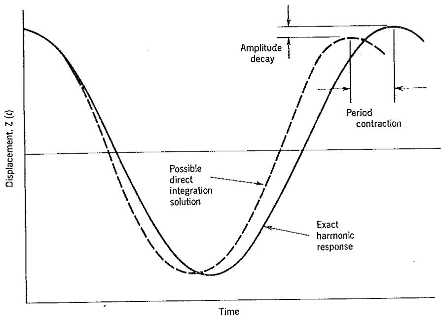
where $\tilde{C}_{1}$ and $\tilde{C}_{2}$ are determined from initial conditions, and $i = \sqrt{-1}$ . The approximate solution obtained by direct integration may display amplitude error and period error. Amplitude error can be either amplitude increase, which is the same as instability, or amplitude decay, which is more commonly called artificial damping or viscosity. Period error can be either period elongation or period contraction. These errors are shown in Fig. 13.13-1.
Because $\lambda_{1}$ and $\lambda_{2}$ are complex conjugates (in both the central-difference and trapezoidal-rule methods), $\mu_{1}$ and $\mu_{2}$ in Eq. 13.13-4 are also complex conjugates and can be written as
$$
\mu_ {1} = a + i b \quad \text { and } \quad \mu_ {2} = a - i b \tag {13.13-16}
$$
where $a$ and $b$ are real. By use of Eq. 13.13-16, Eq. 13.13-4 can be written as
$$
\lambda_ {1} ^ {n} = e ^ {a n \Delta t} e ^ {i b n \Delta t} = e ^ {a n \Delta t} (\cos b n \Delta t + i \sin b n \Delta t) \tag {13.13-17a}
$$
line
| Time Segment | Displacement, Z(t) |
| ------------------------- | ------------------ |
| Exact harmonic response | Minimum |
| Period contraction | Maximum |
| Possible direct integration solution | Minimum |
| Amplitude decay | Maximum |
Figure 13.13-1. Possible errors in direct integration.
$$
\lambda_ {2} ^ {n} = e ^ {a n \Delta t} e ^ {- i b n \Delta t} = e ^ {a n \Delta t} (\cos b n \Delta t - i \sin b n \Delta t) \tag {13.13-17b}
$$
in which the latter forms are obtained by use of DeMoivre's theorem. Combination of Eqs. 13.13-17 and 13.13-3a provides the exact solution to the central-difference approximation:
$$
Z _ {n} = C _ {1} e ^ {a n \Delta t} (\cos b n \Delta t + i \sin b n \Delta t) + C _ {2} e ^ {a n \Delta t} (\cos b n \Delta t - i \sin b n \Delta t) \tag {13.13-18}
$$
Comparison of Eqs. 13.13-15 and 13.13-18 shows that amplitude error will result unless a = 0 and period error will result unless $b = \omega$ .
We define period error, $P$ , by
$$
P = \frac {2 \pi / b}{2 \pi / \omega} = \frac {\omega}{b} \tag {13.13-19}
$$
where $2\pi/\omega$ and $2\pi/b$ are respectively the period of the actual system and the period of the system created by the time integration algorithm. The following types of error are possible:
$$
P > 1 \quad \text { period elongation }
$$
$$
P = 1 \quad \text { no period error }
$$
$$
P < 1 \quad \text { period contraction }
$$
To determine b, we note from Eq. 13.13-17a with n = 1 that
$$
\frac {\mathrm{Im} (\lambda)}{\mathrm{Re} (\lambda)} = \frac {\sin b \Delta t}{\cos b \Delta t} = \tan b \Delta t \tag {13.13-20}
$$
For the central-difference method, Eqs. 13.13-7 and 13.13-20 give the period, b, of the numerically integrated solution as
$$
b = \frac {1}{\Delta t} \tan^ {- 1} \frac {\omega \Delta t \sqrt {4 - \omega^ {2} \Delta t ^ {2}}}{2 - \omega^ {2} \Delta t ^ {2}} \tag {13.13-21}
$$
Combination of Eqs. 13.13-19 and 13.13-21 yields the period error of the central-difference method as
$$
P = \omega \Delta t \left[ \tan^ {- 1} \frac {\operatorname{Im} (\lambda)}{\operatorname{Re} (\lambda)} \right] ^ {- 1} = \omega \Delta t \left[ \tan^ {- 1} \frac {\omega \Delta t \sqrt {4 - \omega^ {2} \Delta t ^ {2}}}{2 - \omega^ {2} \Delta t ^ {2}} \right] ^ {- 1} \tag {13.13-22}
$$
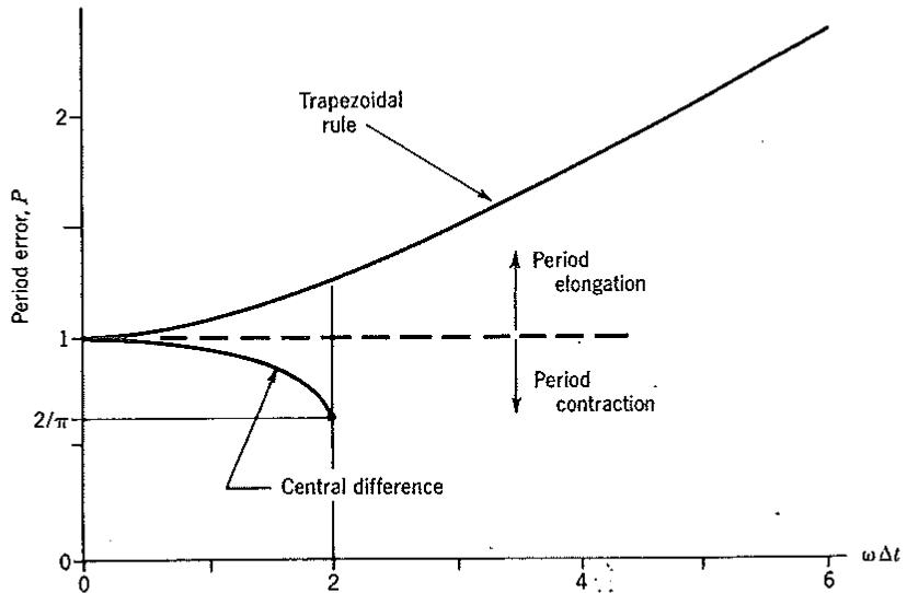
in which the arctangent function is required to yield a positive angle. Equation 13.13-22 represents period contraction and is plotted in Fig. 13.13-2. For the trapezoidal rule, Eqs. 13.13-14, 13.13-19, and 13.13-20 give the period error
$$
P = \omega \Delta t \left[ \tan^ {- 1} \frac {4 \omega \Delta t}{4 - \omega^ {2} \Delta t ^ {2}} \right] ^ {- 1} \tag {13.13-23}
$$
in which the arctangent function is required to yield a positive angle. This represents period elongation and is plotted in Fig. 13.13-2.
Figure 13.13-2 suggests guidelines for mass-matrix selection in direct integration. Natural frequencies obtained by use of consistent mass matrices are overestimated. Hence the periods of modes are underestimated, or contracted. When consistent mass matrices are used with the trapezoidal rule, which has period elongation, period errors in the direct integration of the equations of motion are partially compensatory. This observation is true of implicit methods in general. Use of lumped mass matrices usually underestimates natural frequencies and hence overestimates, or elongates, periods. When lumped mass matrices are used with the central-difference method, period errors are partially compensatory. This observation is also true of explicit methods in general.
line
| ωΔt | Period error, P |
| --- | --- |
| 0 | 1 |
| 2 | 2/π |
| 6 | >2 |
Figure 13.13-2. Period errors for the central-difference and trapezoidal-rule methods.
We emphasize that Fig. 13.13-2 pertains to the mode whose frequency is $\omega$ . A multi-d.o.f. structure has many modes. For structural analysis one selects a $\Delta t$ such that $\omega \Delta t$ is small for all modes of practical interest.
The following amplitude errors are possible:
$$
a > 0 \quad \text { amplitude growth (instability) }
$$
$$
a = 0 \quad \text { no amplitude error }
$$
$$
a < 0 \quad \text { amplitude decay (artificial damping) }
$$
Neither the central-difference nor the trapezoidal-rule method has amplitude error. This can be seen immediately by noting that, when integration is stable, Eq. 13.13-3a applies, and $\left|\lambda_{1}\right|=\left|\lambda_{2}\right|=1$ (although $\lambda_{1}\neq\lambda_{2}$ ). Hence, Eq. 13.13-3a shows that, although $Z_{n}$ may be periodic, it will not grow or decay.
To show in a more formal manner that the central-difference method does not have amplitude error, we consider the sum $\lambda_1 + \lambda_2$ as given by Eqs. 13.13-7 and 13.13-17 with $n = 1$ . This provides
$$
e ^ {a \Delta t} \cos b \Delta t = 1 - \frac {1}{2} \omega^ {2} \Delta t ^ {2} \tag {13.13-24}
$$
Combining Eq. 13.13-24 with Eq. 13.13-21 provides
$$
a \Delta t = \ln \frac {1 - \omega^ {2} \Delta t ^ {2} / 2}{\cos \left[ \tan^ {- 1} \frac {\omega \Delta t \sqrt {4 - \omega^ {2} \Delta t ^ {2}}}{2 - \omega^ {2} \Delta t ^ {2}} \right]} \tag {13.13-25}
$$
Evaluation of Eq. 13.13-25 for $0 \leq \omega \Delta t < 2$ shows that $a \Delta t = 0$ , thus verifying that the central-difference method has no amplitude error. However, this does not imply that the amplitude of response as predicted by the central-difference method will agree with the exact response. This is particularly true when using stable time steps that are very close to the stability limit. To show this, consider Eqs. 13.13-15 and 13.13-18. When $\lambda_{1}$ and $\lambda_{2}$ are distinct, $C_{1}$ and $C_{2}$ in Eq. 13.13-18 are close approximations of $\widetilde{C}_{1}$ and $\widetilde{C}_{2}$ in Eq. 13.13-15. When $\Delta t$ is very close to the stability limit, $\lambda_{1}$ and $\lambda_{2}$ are almost equal and the expressions within the parentheses of Eq. 13.13-18 are almost linear combinations of one another. In this situation, $C_{1}$ and $C_{2}$ may differ greatly from $\widetilde{C}_{1}$ and $\widetilde{C}_{2}$ . In fact, it is for this reason that the “beating” phenomenon of Fig. 13.10-5 is displayed when $\Delta t$ is very close to the stability limit. What is implied by the statement of zero-amplitude error is that the envelope of the numerical solution has a mean value that does not grow or decay in comparison with the exact solution.
Following the same procedure used for the central-difference method, we obtain, for the trapezoidal rule,
$$
a \Delta t = \ln \frac {4 - \omega^ {2} \Delta t ^ {2}}{(4 + \omega^ {2} \Delta t ^ {2}) \cos \left[ \tan^ {- 1} \left(\frac {4 \omega \Delta t}{4 - \omega^ {2} \Delta t ^ {2}}\right) \right]} \tag {13.13-26}
$$
which gives $a \Delta t = 0$ for all values of $\omega \Delta t$ , and therefore implies zero-amplitude error.
# 13.14 CONCLUDING REMARKS ON TIME-HISTORY ANALYSIS
Choice of Method. The choice of method for time-history analysis is strongly problem-dependent. The efficiency of a given method depends on whether the problem is of a wave propagation or a structural dynamics type, the time span for which analysis is required, whether response is linear or nonlinear, and the topology of the finite element mesh.
In wave propagation problems the excitation is usually rich in high-frequency components. Time scales of interest are short and of the order of the acoustic wave traversal time across a structure. Usually we are interested in observing the passage of stress waves through elements and the transients produced. In structural dynamics problems, the excitation and response are characterized by low-frequency, long-time-scale components. Analysis duration is usually long compared to that normally required for a wave propagation problem.
Modal superposition methods are economical when only a small portion of the total number of vibration modes of a model need be used for superposition. Wave propagation problems would require a very large number of modes to be included. Therefore, superposition methods are generally not appropriate for wave propagation problems. In structural dynamics problems, excitation and structural response are dominated by low-frequency components; hence superposition methods can be very effective.
If material response becomes nonlinear or deformations become large, a structure's eigenvalues and eigenvectors change. Because of the expense of solving eigenproblems, it is not prudent to continuously update eigenpairs during nonlinear response. Rather, most modal methods for nonlinear problems treat nonlinearities by pseudoload techniques in which loads that account for nonlinearities are transferred to the right-hand side of the equation of motion. These methods are not robust. Convergence is strongly problem-dependent and is often poor. Generally speaking, direct integration methods are preferable for nonlinear problems.
With explicit methods of direct integration, stability typically requires that the time step be small enough that information does not propagate across more than one element per time step (e.g., the CFL condition). Explicit methods are ideal for wave propagation problems in which behavior at the stress wave front is of engineering importance. Here the stability restriction is not a serious disadvantage because a small $\Delta t$ is necessary for accuracy. Other factors in favor of explicit time integration are easy implementation, accurate treatment of general nonlinearities, and the capability of treating very large problems with only modest computer storage requirements. For structural dynamics problems, time scales and analysis durations are usually long and accuracy considerations alone would permit a $\Delta t$ much larger than the upper limit of $\Delta t$ for stable explicit integration. Although explicit methods are often used for structural dynamics problems, they are not as well suited to this class of problems as they are to wave propagation problems.
The only advantage of implicit methods over explicit methods is that they allow a much larger $\Delta t$ because they are unconditionally stable (conditionally stable implicit methods are not often used). Implicit methods are expensive for wave propagation problems since accuracy requires a small $\Delta t$ . For long-duration structural dynamics problems, implicit methods are usually more effective than explicit methods, although this depends on mesh topology and severity of nonlinearities.
Compared with explicit methods, implicit methods are more difficult to implement, particularly for nonlinear problems, and they require considerably more computer storage.
Choice of Element and Mesh. When discretizing a structure or a medium, an analyst can choose from simple, low-order elements such as the linear-displacement bar, quadratic beam, and bilinear quadrilateral, or from higher-order elements such as the quadratic Lagrange and serendipity quadrilaterals. In wave propagation problems, discontinuities of strain propagate throughout the model. Lower-order displacement elements are more adept at modeling these discontinuities than are higher-order elements, which tend to produce more numerical noise. Structural dynamics problems tend to have strain fields that vary smoothly with time. Hence, higher-order elements can be used to more advantage than in wave propagation problems. Higher-order elements can also be used effectively in eigenvalue problems.
Guidelines discussed in Chapter 19 for construction of finite element meshes for quasistatic problems are also useful for dynamic problems. Thus, static or dynamic stress analysis requires a finer mesh (particularly near stress raisers) than does quasistatic deflection analysis or calculation of lower vibration frequencies. A dynamic problem may require more elements than the analogous quasistatic problem. For example, in the problem of Fig. 13.10-2, only one linear-displacement bar element is necessary for the quasistatic solution, whereas many more elements are necessary to capture the essential features of the dynamic problem or to calculate accurate natural frequencies and mode shapes.
Element sizes should not change abruptly. If they do, the mass matrix will be a poor discrete representation of the actual continuous mass distribution of the structure. This gives rise to artificial wave reflections and additional numerical noise when waves cross boundaries between elements of markedly different size.
With explicit methods, a lumped mass matrix is preferred for reasons of economy and accuracy. With implicit methods, a consistent mass matrix is preferred for accuracy and is only slightly detrimental to economy.
# PROBLEMS
# Section 13.1
13.1 A single d.o.f. spring–mass system has natural frequency $\omega_{1} = \sqrt{k/m}$ . It is excited by a force $P_{0} \sin \omega_{2} t$ . What is the limiting value of the ratio $\omega_{2}/\omega_{1}$ such that the amplitude of motion differs from the static displacement by less than 10%?
# Section 13.2
13.2 Show that under constant acceleration $\{\ddot{d}\}$ , nodal “loads” $[m]\{\ddot{d}\}$ with $[m]$ given by Eq. 13.2-5 are the same as the body force nodal loads given by Eq. 4.1-6.
# Section 13.3
13.3 (a) Can a diagonal coefficient in a consistent mass matrix ever be negative? Explain.
(b) Imagine that a beam is vibrated so that nodes of the vibration mode coincide with nodes of the finite element mesh. Would you prefer the consistent mass matrix of Eq. 13.3-2 or the lumped mass matrix of Eq. 13.3-3 with $\alpha = 0$ ? Is Eq. 13.3-3 with $\alpha \neq 0$ an acceptable alternative?
13.4 (a) Derive the consistent mass matrix given by Eq. 13.3-1.
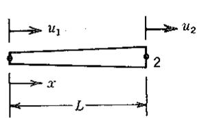
(b) Imagine that the cross-sectional area of the bar shown in the figure varies linearly from area $A_{0}$ at the left end to area $\gamma A_{0}$ at the right end, where $\gamma$ is a constant. Determine the consistent mass matrix associated with d.o.f. $u_{1}$ and $u_{2}$ .
(c) Show that [m] and [m] in Eq. 13.3-1 each yield the correct nodal forces under a rigid-body translational acceleration in the bar's axial direction.
text_image
u₁
u₂
2
x
L
Problem 13.4
text_image
u₁
2
u₂
3
u₃
1
x
L
2
L
2
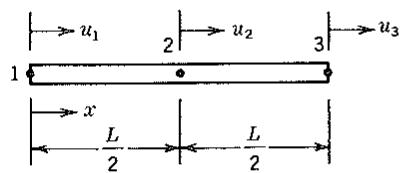
Problem 13.7
13.5 (a) Derive the consistent mass matrix given by Eq. 13.3-2.
(b) Show that Eq. 13.3-2 yields the correct nodal forces and moments under a rigid-body translational acceleration transverse to the axis of the beam.
13.6 Determine the consistent mass matrix of the constant-strain triangle (Fig. 4.2-3). The element has uniform density and thickness. Arrange d.o.f. in the order $\{\mathbf{d}\} = \left[u_1 u_2 u_3 v_1 v_2 v_3\right]^T$ .
13.7 (a) Derive the consistent mass matrix that operates on d.o.f. $u_{1}, u_{2}$ and $u_{3}$ for the uniform quadratic-displacement bar shown.
(b) Using heuristic arguments, derive an ad hoc lumped matrix for this element that agrees with HRZ lumping (Eq. 13.3-9).
13.8 Determine $\alpha$ in Eq. 13.3-3 such that the beam element has the correct kinetic energy $I\omega^2 / 2$ under rigid-body rotation about its center. Then consider modeling a simply supported beam with one element and computing the natural frequencies of vibration. What conclusions can you draw from this problem?
13.9 For the HRZ mass-lumping procedure:
(a) Verify Eqs. 13.3-4 and 13.3-5.
(b) Verify the nodal masses shown in parentheses for the element shown in Fig. 13.3-3a.
(c) Verify the nodal masses shown in parentheses for the element shown in Fig. 13.3-3b.
(d) Determine the lumped mass matrix $\lceil \mathbf{m} \rceil$ for the constant-strain triangle element of Problem 13.6. Consider $x$ - and $y$ -direction accelerations separately.
13.10 For optimal lumping by quadrature verify the nodal masses for the following elements shown in Fig. 13.3-4.
(a) The quadratic-displacement (six-node) triangle.
(b) The quadratic-displacement Lagrange (nine-node) quadrilateral.
13.11 For a uniform beam element having the usual four d.o.f. (see, e.g., Fig. 13.3-1b), consider the lateral-displacement field
$$
w = \left\lfloor (1 - \xi), (\xi - \xi^ {2}) L / 2, \xi , (- \xi + \xi^ {2}) L / 2 \right\rfloor \left\lfloor w _ {1} \quad \theta_ {1} \quad w _ {2} \quad \theta_ {2} \right\rfloor^ {T}
$$
where $\xi = x / L$ .
(a) Show that $w$ is linear in $x$ if $\theta_1 = \theta_2$ . Also show that this field yields the correct displacement $w$ and curvature $w_{,xx}$ under pure bending.
(b) Use Eq. 13.2-5 to evaluate the mass matrix.
(c) Obtain a diagonal mass matrix by applying the HRZ procedure.
# Section 13.4
13.12 (a) Determine the Rayleigh proportional damping constants $\alpha$ and $\beta$ for fractions of critical damping of 3% and 20% at frequencies of 5 and 15 Hz, respectively.
(b) For the values of $\alpha$ and $\beta$ determined in part (a), draw a graph similar to Fig. 13.4-1. Comment on the fraction of critical damping experienced by frequencies below 5 Hz and above 15 Hz. Is caution called for?
13.13 Consider a particle that is allowed to free-fall from at-rest initial conditions under its own weight due to gravity. If the particle has mass-proportional damping, then the equation governing its velocity v is $\dot{v} + \beta v = g$ , where g is the acceleration due to gravity. (Remark: The same equation governs the velocity of a particle allowed to sink in a viscous fluid where $\beta$ is related to a fluid viscosity.)
(a) Determine the analytic solution for v.
(b) Consider the ratio of the damped velocity to the undamped velocity (i.e., $v_{\text{undamped}} = gt$ ) for values of $t$ of about 1 second. Does this ratio offer guidelines on what values of $\beta$ are permissible without excessively damping rigid-body modes?
# Section 13.5
13.14 (a) Show that the Rayleigh quotient, Eq. 13.5-4, can be regarded as stating an equality between the maximum strain and kinetic energies associated with mode $\{\overline{\mathbf{D}}\}$ .
(b) Imagine that redesign produces small changes in [M] and [K]. Hence, the natural frequency $\lambda_{i}$ of each mode $\{\overline{\mathbf{D}}\}_{i}$ is slightly changed, by an amount $\Delta \lambda_{i}$ . Using the Rayleigh quotient and neglecting terms of higher order, derive an expression for $\Delta \lambda_{i}$ in terms of $\lambda_{i}$ , $\{\overline{\mathbf{D}}\}_{i}$ , [M], [ΔK], and [ΔM].
13.15 (a) Prove that the lower inequality of Eq. 13.5-5 is true. Suggestion: Express $\{\mathbf{v}\}$ as a linear combination of eigenvectors (each normalized as in Eq. 13.6-2), factor the common term $\lambda_{\min}$ out of the numerator, and argue that when $\{\mathbf{v}\} \neq \{\overline{\mathbf{D}}_{\min}\}$ the numerator is too large and hence overestimates $\lambda_{\min}$ .
(b) Prove that the upper inequality of Eq. 13.5-5 is true.
13.16 Consider the following stiffness and mass matrices:
$$
[ \mathbf {K} ] = \left[ \begin{array}{c c} 2 & - 2 \\ - 2 & 5 \end{array} \right] \quad [ \mathbf {M} ] = \left[ \begin{array}{c c} 1 & 0 \\ 0 & 1 \end{array} \right]
$$