Exact eigenvalues and eigenvectors for axial vibration are $\lambda_1 = 1$ , $\lambda_2 = 6$ , $\{\overline{\mathbf{D}}\}_1 = [2 - 1]^T$ , and $\{\overline{\mathbf{D}}\}_2 = [1 - 2]^T$ . Consider approximate eigenvectors $[1.7 - 1.0]^T$ and $[1.2 - 2.0]^T$ and show that the Rayleigh quotient provides an accurate estimate of $\lambda_1$ and $\lambda_2$ .
13.17 Consider axial vibrations of a uniform bar of length L and mass $m = \rho AL$ , free at one end and fixed at the other. Using two-node bar elements, model the bar first by one element, then by two elements of equal length L/2. In each case, compute the lowest natural frequency using
(a) the consistent mass matrix [m].
(b) the lumped mass matrix [m].
(c) the average mass matrix ([m] + [m])/2.
The exact lowest natural frequency is $\omega_{\mathrm{I}} = (\pi /2L)\sqrt{E / \rho}$ .
13.18 In Problem 13.17 consider the convergence rates of $\lambda_{\mathrm{min}}$ as the mesh is refined. Are they in accord with the rates predicted in Section 13.3?
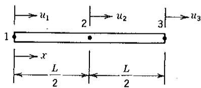
13.19 The stiffness, consistent mass, and optimally lumped mass matrices for the unsupported, uniform, three-node quadratic bar element shown are
$$
\frac {A E}{3 L} \left[ \begin{array}{r r r} 7 & - 8 & 1 \\ - 8 & 1 6 & - 8 \\ 1 & - 8 & 7 \end{array} \right], \quad \frac {\rho A L}{3 0} \left[ \begin{array}{r r r} 4 & 2 & - 1 \\ 2 & 1 6 & 2 \\ - 1 & 2 & 4 \end{array} \right], \quad \frac {\rho A L}{6} \left[ \begin{array}{r r r} 1 & 0 & 0 \\ 0 & 4 & 0 \\ 0 & 0 & 1 \end{array} \right]
$$
(a) For axial vibration, determine the three natural frequencies and mode shapes using the consistent mass matrix.
(b) Repeat part (a) using the optimally lumped mass matrix.
(c) What is the physical significance of the lowest frequency and mode for parts (a) and (b)?
(d) The exact frequencies of an unsupported continuous bar of length $L$ are $\omega_{n} = (n\pi / L) \sqrt{E / \rho}$ ; $n = 0, 1, 2, \ldots$ . What are the percentage errors of the frequencies computed in parts (a) and (b)?
text_image
u₁
2 → u₂
3 → u₃
1
x
L
2
L
2
Problem 13.19
13.20 Fix one end of the three-node bar treated in Problem 13.19. Determine the two natural frequencies and mode shapes of axial vibration.
(a) Use the consistent mass matrix.
(b) Use the optimally lumped mass matrix.
(c) Use ad hoc lumping in which particles of mass $\rho AL/3$ are placed at each node.
(d) For parts (a), (b), and (c), estimate the lowest frequency by means of the Rayleigh quotient and the assumed displacement mode $u_{1} = 0$ , $u_{2} = 1$ , and $u_{3} = 2$ .
13.21 Model a simply supported uniform beam of length 2L by a single element. Determine the natural frequencies of vibration, where possible, by using
the mass matrices cited here. Use the element stiffness matrix given in Eq. 4.2-5. The exact fundamental frequency is $\omega_{1} = (\pi^{2}/4L^{2})\sqrt{EI/\rho A}$ .
(a) The consistent mass matrix [m] for a bar element given by the first of Eqs. 13.3-1 with d.o.f. $u_{1}$ and $u_{2}$ discarded.
(b) The consistent mass matrix [m] for a beam element given by Eq. 13.3-2.
(c) The lumped mass matrix $\lceil \mathbf{m} \rfloor$ are given by Eq. 13.3-3 with $\alpha = 0$ .
(d) Repeat part (c) with $\alpha = 17.5$ .
(e) The lumped mass matrix $\lceil m \rceil$ given by Eq. 13.3-5.
(f) The matrix [m] given by Problem 13.11(b).
13.22 Consider a uniform cantilever beam of length $L$ , modeled by a single beam element. Repeat parts (a) through (f) of Problem 13.21. The exact fundamental frequency is $\omega = (3.516 / L^2) \sqrt{EI / \rho A}$ .
13.23 A uniform beam is clamped at both ends. In order to exploit geometric symmetry, only the left half of the beam is modeled for vibration analysis. How would you ensure that analysis of the left half yields all natural frequencies of the original clamped-clamped beam?
# Section 13.6
13.24 (a) Verify Eqs. 13.6-1.
(b) Explain a procedure for normalizing a vector (as, for example, $\{\overline{\mathbf{D}}\}_i$ is normalized with respect to [M] in Eq. 13.6-2).
(c) Show that Eqs. 13.6-1 are true for the modes stated in Eqs. 13.5-10.
(d) Show that Eqs. 13.6-1 are true for the exact modes stated in Problem 13.16.
13.25 Verify Eq. 13.4-2. Suggestion: Compare the uncoupled equation of motion with Rayleigh damping to the single d.o.f. equation $\ddot{Z} + 2\xi\omega\dot{Z} + \omega^{2}Z = p$ .
13.26 Consider the stiffness and lumped mass matrices given in Problem 13.16. Derive the system of uncoupled ordinary differential equations for a mode displacement response analysis.
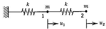
13.27 (a) Let $k = m = 1$ in the spring-mass system shown. Let this system be set in axial motion with initial conditions $u_{1} = u_{2} = \dot{u}_{1} = 0, \dot{u}_{2} = 1$ . Compute $u_{1}$ and $u_{2}$ at times $t = 1, 2, 3, 4$ , and 5 by use of the mode displacement method. Include both modes of the original system in $[\phi]$ . (b) What is the greatest percentage error in $u_{1}$ and $u_{2}$ if only the lowest mode is used, so that $[\phi]$ becomes a column vector?
text_image
k
m
k
m
1
2
→ u₁
→ u₂
Problem 13.27
13.28 Verify Eq. 13.6-11. Suggestion: Insert $[\phi]^{-T}[\phi]^T$ after $[\mathbf{K}]^{-1}$ in the second term of Eq. 13.6-10. Then use orthogonality and the relation $[\phi]^{-1}[\mathbf{K}]^{-1} = [\omega^2]^{-1}[\phi]^T$ to obtain Eq. 13.6-11.
13.29 Consider the two-spring, two-mass system described in Problem 13.27. Let this system be undeformed and at rest at time $t = 0$ . For each of the
following two loadings, use the mode displacement method and then the mode acceleration method to determine $u_{1} = u_{1}(t)$ and $u_{2} = u_{2}(t)$ . Retain only the lowest mode $\{\phi\}_{1}$ in the transformation. Compute numerical values of $u_{1}$ and $u_{2}$ at times t = 2, 4, 6, 8, and 10.
(a) Node 1 is not loaded. A force $F_{2} = 1$ is applied to node 2 at $t = 0$ .
(b) Forces $F_{1} = 1$ and $F_{2} = -1$ are applied to nodes 1 and 2 respectively at $t = 0$ .
13.30 Show that the mode acceleration method reduces to the mode displacement method if the structure moves freely—that is, with $\{R^{ext}\} = \{0\}$ .
13.31 Consider applying a Ritz vector analysis to the system of two springs and two masses described in Problem 13.27.
(a) Externally applied loads are zero so arbitrarily assign $\{\mathbf{w}^{*}\}_{1} = [1 - 0]^{T}$ in Table 13.6-1. Hence, establish a 2 by 2 array [W] of Ritz vectors and the transformed system of Eq. 13.6-18.
(b) Repeat part (a), now using $\{\mathbf{w}^{*}\}_{1} = [0 - 1]^{T}$ .
(c) If $\{\mathbf{w}^{*}\}_{1}$ is arbitrarily taken as $[1 - 2]^{T}$ , and no additional vectors are used, what is the resulting form of Eq. 13.6-18? What fundamental frequency $\omega$ does this equation yield? By what other name do you know this method of calculating $\omega$ ?
# Section 13.7
13.32 Mass condensation, starting from Eq. 13.7-1, would be more accurate if the assumption $[M_{ms}] = [M_{ss}] = [0]$ were not made. What is an objection to this approach?
13.33 (a) Show that Eq. 13.7-5 yields $[\mathbf{K}_r] = [\mathbf{K}_{mm}] - [\mathbf{K}_{ms}][\mathbf{K}_{ss}]^{-1}[\mathbf{K}_{ms}]^T$ . Where has the relation been seen before?
(b) Derive a similar expression for $[M_{r}]$ from Eq. 13.7-5.
13.34 If $\lambda[\mathbf{M}]\{\overline{\mathbf{D}}\}$ in Eq. 13.5-2 is regarded as a vector of inertia loads $\{\mathbf{R}\}$ , and $[\mathbf{K}]$ is inverted to become the flexibility matrix $[\mathbf{F}]$ , we can write $[\mathbf{F}]\{\mathbf{R}\} = \{\mathbf{D}\}$ .
(a) Partition this equation into $m$ master and $s$ slave d.o.f. as in Eq. 13.7-1 and let $\{\mathbf{R}_s\} = \{\mathbf{0}\}$ . Derive the transformation
$$
\left\{ \begin{array}{l} \overline {{\mathbf {D}}} _ {m} \\ \overline {{\mathbf {D}}} _ {s} \end{array} \right\} = [ \mathbf {T} ] \{\overline {{\mathbf {D}}} _ {m} \}, \quad \text { where } \quad [ \mathbf {T} ] = \left[ \begin{array}{l} \mathbf {I} \\ \mathbf {F} _ {m s} ^ {T} \mathbf {F} _ {m m} ^ {- 1} \end{array} \right]
$$
(b) Show that this transformation is mathematically the same as that of Eq. 13.7-3.
(c) How can $[\mathbf{F}_{mm}]$ be computed from [K] and what is its physical meaning?
(d) Why is the transformation of part (a) likely to be more computationally efficient than the form used in Eq. 13.7-3?
13.35 Consider the two-d.o.f. unsupported bar of Fig. 13.5-1. What is the reduced stiffness matrix that results from taking $u_{2}$ as a slave d.o.f.? Is this result reasonable?
13.36 Consider application of the procedure for automatic selection of master d.o.f. described in Section 13.7 to the structure shown. Only axial motion is permitted. Recall from Section 2.11 that condensation of a d.o.f. places

text_image
k
m
k
m
k
m
k
m
k
m
1
2
3
4
5
x, u
Problem 13.36
the two adjacent springs in series. To simplify this problem, but for no sound theoretical reason, assume that condensation of a mass m effectively adds mass m/2 to the two adjacent masses, so that [M] remains diagonal. For the structure shown,
(a) choose two masters by making three left-to-right sweeps.
(b) choose two masters by making three right-to-left sweeps.
(c) determine the frequencies $\omega_{1}$ and $\omega_{2}$ in parts (a) and (b) and compare results. The exact first two frequencies for the five-d.o.f. structure are $0.2846\sqrt{k/m}$ and $0.8308\sqrt{k/m}$ .
13.37 (a) The frequency $\omega_1^2 = 6.1765EI / mL^3$ is computed below Eq. 13.7-12 in the example that closes Section 13.7. Improve this estimate, if possible, by using $\overline{w}_1 = 1$ and the first $\overline{\theta}_2$ of Eq. 13.7-13 in the Rayleigh quotient (Eq. 13.5-4). Use [K] and [M] from Eq. 13.7-8.
(b) Repeat part (a) using the second $\bar{\theta}_2$ of Eq. 13.7-13.
13.38 (a) In the example problem that closes Section 13.7, is the choice of $\overline{w}_1$ as master and $\overline{\theta}_2$ as slave consistent with the rule of largest $M_{ii} / K_{ii}$ ?
(b) Make the other choice, $\bar{\theta}_{2}$ as master and $\overline{w}_{1}$ as slave, and compute the frequency and mode shape (analogous to Eqs. 13.7-12 and 13.7-13).
(c) Improve the estimate of $\omega_{1}$ from part (b) by using its mode shape in the Rayleigh quotient, Eq. 13.5-4, with [K] and [M] taken from Eq. 13.7-8.
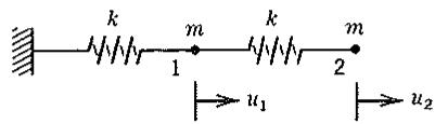
13.39 Apply mass condensation to the system shown. Only axial motion is permitted. Let $k = 1$ and $m = 2$ . Determine the fundamental vibration frequency of the reduced system and compare it with the exact value for the original system. Determine the fundamental mode of the reduced system, using first Eq. 13.7-3 and then Eq. 13.7-7. Finally, obtain improved estimates of $\omega_{1}$ by using each of these modes in the Rayleigh quotient.
text_image
k
m
k
m
1
2
→ u₁
→ u₂
Problem 13.39
13.40 Many methods of solving large eigenproblems require factoring either the stiffness matrix or a combination of the stiffness and mass matrices (e.g., the determinant search and subspace iteration methods). Factoring requires approximately $n_{eq}b^{2}/2$ operations (i.e., multiplications) where $n_{eq}$ is the number of equations and b is the semibandwidth. For full matrices, the number of operations is about $n_{eq}^{3}/6$ . Consider a system of 5000 equations with b = 500. If this system of equations is partitioned into m master and s slave d.o.f., what must m be so that factoring the condensed (full) system is no more expensive than factoring the original (banded) system? What if b = 100 instead?
# Section 13.8
13.41 Repeat the example that closes Section 13.8 using only the first vector of assembled component normal modes plus the additional mode that accounts for having node 3 fixed in the component mode analyses (i.e., omit the second column of Eq. 13.8-12 and the second column of Eq. 13.8-14).
13.42 Consider axial vibration of the spring–mass system shown with k = 1 and m = 1. Natural frequencies are $\omega_{1} = 0.9246$ , $\omega_{2} = 1.574$ , and $\omega_{3} = 2.381$ . Create one substructure consisting of the springs to the left of node 2 and another substructure consisting of the springs to the right of node 2. Using component mode synthesis, determine the two natural frequencies of the reduced structure.
(a) Use method CMS1, following the example in the text.
(b) Repeat part (a) except omit the last Ritz vector obtained by applying a unit load to node 2 (only one frequency can be determined).
(c) Use method CMS2, following the example in the text.
(d) Repeat part (c) except omit the last Ritz vector obtained by applying a unit displacement to node 2 (only one frequency can be determined).

text_image
k m k m 2k m 2k
1 2 3
Problem 13.42
13.43 Repeat Problem 13.42, but let each of the four springs have stiffness $k = 1$ . Natural frequencies and mode shapes of the original structure are
$$
\begin{array}{l} \omega_ {1} = 0. 7 6 5 4 \quad \{\overline {{{\mathbf {D}}}} \} _ {1} = \left[ \begin{array}{l l l} 1 & \sqrt {2} & 1 \end{array} \right] ^ {T} \\ \omega_ {2} = 1. 4 1 4 \quad \{\overline {{{\mathbf {D}}}} \} _ {2} = \left[ - 1 0 1 \right] ^ {T} \\ \omega_ {3} = 1. 8 4 8 \quad \{\overline {{{\mathbf {D}}}} \} _ {3} = \left\lfloor 1 - \sqrt {2} 1 \right] ^ {T} \\ \end{array}
$$
In some cases, a frequency of the original structure may be missing from the reduced structure. Why?
# Section 13.9
13.44 The forward and backward Euler direct integration methods are defined by
$$
\begin{array}{l} \{\mathbf {D} \} _ {n + 1} = \{\mathbf {D} \} _ {n} + \Delta t \{\dot {\mathbf {D}} \} _ {n} \quad \text { forward Euler } \\ \{\mathbf {D} \} _ {n + 1} = \{\mathbf {D} \} _ {n} + \Delta t \{\dot {\mathbf {D}} \} _ {n + 1} \quad \text { backward Euler } \\ \end{array}
$$
Are these methods explicit or implicit?
# Section 13.10
13.45 Using the Taylor series expansion, determine the order of accuracy of the direct integration methods defined in Problem 13.44.
13.46 Verify Eq. 13.10-12.
13.47 Show that Eq. 13.10-12 reduces to Eq. 13.10-5 if damping is zero.
13.48 (a) Apply the Gerschgorin bound, Eq. 13.10-17, with element coefficients replaced by structure coefficients and $n_e$ replaced by $n_{\mathrm{eq}}$ , to obtain a
bound on the maximum mesh frequency in terms of $E$ , $\rho$ , and $L$ for the model and boundary conditions shown in Fig. 13.10-2. Then divide the bar into 40 elements of equal length and evaluate the bound numerically. (b) Show that the bound obtained in part (a) agrees precisely with the element bound, Eq. 13.10-15. (Note: Usually the Gerschgorin and element bounds do not agree.)
13.49 Consider a model consisting of one linear-displacement bar finite element, with lumped mass, and one end fixed. Do the Gerschgorin bound, Eq. 13.10-17, and the element bound, Eqs. 13.5-7 and 13.10-15, show good agreement with the exact frequency of this model?
13.50 Consider a uniform free-free bar (i.e., an unsupported bar) modeled by equal-length, linear-displacement finite elements. For such a situation, the maximum frequency of the entire model and the maximum unconstrained element frequency are the same. Why?
13.51 In the example of Section 13.10, the element bound was within one-thousandth of a percent of the maximum mesh frequency. Do you expect the agreement to improve or deteriorate as the number of elements in the mesh increases? Why?
13.52 A particle of unit mass is supported by a spring of unit stiffness. There is no damping and no external load. Thus $k = m = \omega = 1$ . At time $t = 0$ , the particle has zero displacement, zero acceleration, but unit velocity. Use the central-difference method, Eq. 13.10-5, to compute displacement versus time over five time steps. Use a $\Delta t$ of (a) 1.0, (b) $\sqrt{2.0}$ , (c) 2.0, and (d) 3.0. Does there appear to be an amplitude error? Why?
13.53 Repeat the example of Section 13.10 for the bar shown in Fig. 13.10-2 but with the right-hand end unsupported. Modify the Fortran program and compare the displacement, velocity, and stress time histories at the position x = 9.75 in. with those for the bar in Fig. 13.10-2. Experiment with time steps of different size. Also examine the time history solutions for position x = 4.75 in.
13.54 Repeat the example of Section 13.10 with a mesh of nonuniform length elements. For the first 15 in. of the bar, use 30 elements, each of length 0.5 in. For the remaining 5 in. of the bar, use five elements of length 1 in. Compare the velocity and stress time-histories at the position $x = 9.75$ in. with those of the example of Section 13.10 and comment on any differences.
13.55 For central-difference integration of equations of motion with Rayleigh damping, derive an equation analogous to Eqs. 13.10-5 and 13.10-12, and modify the computational procedure of Table 13.10-1. In deriving this algorithm, write the viscous forces as $\alpha[\mathbf{K}]\{\dot{\mathbf{D}}\}_{n-1/2} + \beta[\mathbf{M}]\{\dot{\mathbf{D}}\}_n$ . For the mass-proportional part of the damping, approximate $\{\dot{\mathbf{D}}\}_n$ by Eq. 13.10-1. Note that the stiffness-proportional part of the viscous forces can be obtained element-by-element by summation of the element contributions $\alpha \int [\mathbf{B}]^T\{\dot{\boldsymbol{\sigma}}\}_{n-1/2} dV$ (verify this). Based on Eqs. 13.10-8 and 13.10-14, can you suggest what the stability criterion for this scheme will be?
13.56 Using the damping algorithm developed in Problem 13.55, modify the Fortran program of Fig. 13.10-3 to include Rayleigh damping. Use stiffness-proportional damping to give 20% critical damping at the frequency given by Eq. 13.10-15 and zero mass-proportional damping. Repeat the example
problem of Section 13.10 and compare results. Experiment with different mass- and stiffness-proportional damping constants.
# Section 13.11
13.57 Derive Eq. 13.11-1 using Taylor series and show that $\{D\}_{n+1}$ is approximated with an error of $O(\Delta t^{2})$ . Suggestion: Write Taylor series for $\{D\}_{n+1}$ about time $n \Delta t$ and $\{D\}_{n}$ about time $(n + 1) \Delta t$ and then combine them to obtain Eq. 13.11-1 plus higher-order terms.
13.58 Verify Eqs. 13.11-3 through 13.11-7.
13.59 Why do you think the name “trapezoidal rule” is applied to Eqs. 13.11-1 and 13.11-2?
13.60 Repeat Problem 13.52, using the trapezoidal rule (Table 13.11-1). Use four time steps, of magnitude (a) $\Delta t = 2.0$ , and (b) $\Delta t = 1.0$ .
13.61 In seismic analysis of structures, 30 Hz is usually used as a cutoff frequency; that is, the excitation is composed of components with frequencies lower than 30 Hz. Using this cutoff frequency, what is the largest $\Delta t$ that should be used for an unconditionally stable implicit method to give accurate results?
# Section 13.12
13.62 Show that when $\beta = \frac{1}{4}$ and $\gamma = \frac{1}{2}$ , Eqs. 13.12-3 and 13.12-4 can be expressed as Eqs. 13.11-1 and 13.11-2.
13.63 Why is the term “linear acceleration” used when $\beta = \frac{1}{6}$ in Table 13.12-1?
13.64 (a) Use the explicit Newmark method, Eqs. 13.12-3 and 13.12-4 with $\beta = 0$ , to derive a computational procedure analogous to Table 13.10-1. State whether [M] and [C] must be diagonal.
(b) Does this procedure have any advantages in comparison with the central-difference procedure of Eq. 13.10-5?
13.65 (a) Using the results of Problem 13.64, modify the Fortran program of Fig. 13.10-3 to use the explicit Newmark method ( $\beta = 0, \gamma \geq \frac{1}{2}$ ).
(b) Repeat the example of Section 13.10 using the algorithm of part (a) with $\gamma = 0.5$ (no artificial damping).
(c) Repeat the example of Section 13.10 using the algorithm of part (a) with $\gamma = 0.6, 0.7, 0.8, 0.9, 1.0$ (increasing artificial damping).
13.66 Use the implicit Newmark method, Eqs. 13.12-3 and 13.12-4 with $\beta > 0$ , to derive equations analogous to Eqs. 13.11-5 through 13.11-7.
# Section 13.13
13.67 Consider the uncoupled homogeneous equation of motion with damping but without inertia: $2\xi\omega\dot{Z} + \omega^{2}Z = 0$ . Using spectral stability, determine the stability criterion for direct integration of this equation by:
(a) The central-difference method, Eq. 13.10-1.
(b) The trapezoidal rule. Suggestion: Sum the equation of motion at times $n \Delta t$ and $(n + 1) \Delta t$ and combine with Eq. 13.11-1 to eliminate velocities.
(c) The forward Euler method defined in Problem 13.44.
(d) The backward Euler method defined in Problem 13.44.
13.68 Consider Problem 13.52 again, in which the central-difference method (Eq. 13.10-5) is applied to a spring-mass system for which $k = m = \omega = 1$ . Now use $\Delta t = \sqrt{3.96}$ and start the algorithm using $u_0 = 0$ and $u_{-1} = -1$ . Follow the motion for at least ten cycles, and observe that the computed amplitude displays "beating" but no net growth.
13.69 (a) Derive Eq. 13.13-23.
(b) Derive Eq. 13.13-26.
13.70 (a) Numerically evaluate Eqs. 13.13-22 and 13.13-25 using $\omega \Delta t = 0, 1, \sqrt{2}$ , 2 for the period and amplitude errors of the central-difference method.
(b) Numerically evaluate Eq. 13.13-23 and 13.13-26 using $\omega \Delta t = 0, 1, 2, 4$ for the period and amplitude errors of the trapezoidal rule.
(c) Analytically show that Eqs. 13.13-25 and 13.13-26 reduce to forms that yield $a\Delta t = 0$ for all values of $\omega \Delta t$ .
13.71 Consider the central-difference solutions obtained in Problem 13.52, parts (a), (b), and (c). What is the period error in each case? Check that the values you obtain agree with Eq. 13.13-22.
13.72 Consider the trapezoidal-rule solutions obtained in Problem 13.60, parts (a) and (b). Using approximations as necessary, determine the period and the period error of each solution. Check that the values you obtain agree with Eq. 13.13-23.
# Section 13.14
13.73 The uncoupled equations produced by a modal analysis (Section 13.6) have a lower $\omega_{max}$ than $\omega_{max}$ of the full system. Hence, in integrating the uncoupled equations, what are the relative merits of explicit and implicit methods? How does the specific choice of modal method affect your answer?
# STRESS STIFFENING AND BUCKLING
Bending stiffness is affected by membrane forces. Matrices that account for this effect are formulated and applied to problems such as buckling. The nature of the buckling problem is discussed and warnings given against oversimplification.
# 14.1 INTRODUCTION
Buckling of bars, frames, plates, and shells may occur as a structural response to membrane forces. Membrane forces act along member axes and tangent to plate and shell midsurfaces. The membrane force in a bar (or column) is the axial load. Membrane forces in a shell are defined by Eqs. 12.1-1.
Buckling occurs when a member or a structure converts membrane strain energy into strain energy of bending with no change in externally applied load. A critical condition, at which buckling impends, exists when it is possible that the deformation state may change slightly in a way that makes the loss in membrane strain energy numerically equal to the gain in bending strain energy. In a slender bar of length L, axial stiffness AE/L is much greater than bending stiffness $EI/L^{3}$ . Similarly, in a thin-walled structure such as a shell, membrane stiffness is typically orders of magnitude greater than bending stiffness. Accordingly, small membrane deformations can store a large amount of strain energy, but comparatively large lateral deflections and cross-section rotations are needed to absorb this energy in bending deformations.
One can also take the view that membrane forces alter the bending stiffness of a structure. Thus buckling occurs when compressive membrane forces are large enough to reduce the bending stiffness to zero for some physically possible deformation mode. If the membrane forces are reversed—that is, made tensile rather than compressive—bending stiffness is effectively increased. This effect is called stress stiffening.
The effects of membrane forces are accounted for by a matrix $[k_{\sigma}]$ that augments the conventional stiffness matrix [k]. Matrix $[k_{\sigma}]$ has been given various names, as follows: initial stress stiffness matrix, differential stiffness matrix, geometric stiffness matrix, and stability coefficient matrix. In what follows we give $[k_{\sigma}]$ the name stress stiffness matrix. Matrix $[k_{\sigma}]$ is defined by an element's geometry, displacement field, and state of stress. Thus, $[k_{\sigma}]$ is independent of elastic properties. (However, by introducing the stress–strain relation, $[k_{\sigma}]$ can alternatively be written in terms of elastic properties and strains or deformations.) The structure matrix $[K_{\sigma}]$ is built by summing overlapping terms of element matrices $[k_{\sigma}]$ , in the same way that the conventional [K] is built by summing overlapping terms of element matrices [k].
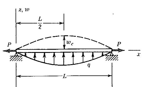
Analysis of a Beam-Column. Consider the simply supported beam shown in Fig.
text_image
z, w
L
2
w_c
P
P
x
q
L
$\{n\}$
text_image
ds = (1 + w_x^2)^(1/2) dx
w_x dx
dx
(b)
Figure 14.1-1. (a) A uniform beam on simple supports. (b) Geometric relations for a differential element of length dx.
14.1-1. Axial force P, positive in tension, is regarded as being imposed at the outset, for example, by cooling the bar while not allowing its ends to move toward one another. We will use energy concepts and a single d.o.f. to illustrate the stiffening effect of axial force P and to derive the buckling load $P_{cr} = -\pi^{2}EI/L^{2}$ , where the negative sign indicates compression.
Strain energy in bending is given by the standard expression that involves the square of curvature $w_{,xx}$ :
$$
U _ {b} = \frac {1}{2} \int_ {0} ^ {L} E I w _ {, x x} ^ {2} d x \tag {14.1-1}
$$
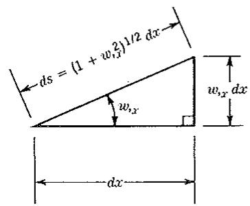
Let a small lateral displacement $w = w(x)$ take place. Thus each differential length dx is changed to a new length ds, where ds > dx because the distance between supports is not allowed to change. From Fig. 14.1-1b,
$$
d s = (1 + w _ {, x} ^ {2}) ^ {1 / 2} d x \approx \left(1 + \frac {w _ {, x} ^ {2}}{2}\right) d x \tag {14.1-2}
$$
where the latter approximation comes from the first two terms of the binomial expansion. The approximation is valid if $w_{;x}^{2}<<1$ , which restricts this development to small rotations. Axial membrane strain in the bar is therefore
$$
\epsilon_ {m} = \frac {d s - d x}{d x} \approx \frac {w _ {, x} ^ {2}}{2} \tag {14.1-3}
$$
In the linear theory of elasticity we ignore terms of order $w_{,x}^{2}$ . But here we seek the consequences of retaining the more important of the higher-order terms that linear theory neglects. We are taking a physical approach to formulating these terms. They may also be obtained by a systematic procedure of linearization, as will be touched upon in Section 14.4.
During a small lateral displacement $w = w(x)$ , axial force P in the bar remains practically constant. As each elemental length dx lengthens an amount $\epsilon_{m}$ dx, the force P it carries does work (and stores membrane strain energy) in the amount $P\epsilon_{m}$ dx. Thus the change in membrane energy is $^{1}$
$^{1}$ The same expression would result from the assumptions of a roller support at the right end, constant P, and constant length ( $\int ds = L$ ), which would cause the right end to move a distance $u_{L} = \int \epsilon_{m} dx$ , so that force P at x = L gains potential in the amount $Pu_{L}$ .