present example, 2m - 1 = 1, which means that d.o.f. of a finite element model would have to include nodal values of $\tilde{u}$ and $\tilde{u}_{,x}$ in order to achieve the required continuity. Integration by parts reduces 2m - 1 to 1 - 1 = 0, so that d.o.f. of a finite element model need only include nodal values of $\tilde{u}$ . Integration by parts also serves to introduce nonessential boundary conditions, as follows. In one dimension, the formula for integration by parts is written in conventional notation as $\int u dv = uv - \int v du$ , where $u$ and $v$ represent functions of $x$ . In the present example, we apply integration by parts to the term $W_{i}\tilde{u}_{,xx}$ only. Thus $W_{i}\tilde{u}_{,xx} dx$ is regarded as $u dv$ in the formula for integration by parts, where $u = W_{i}$ and $dv = \tilde{u}_{,xx} dx = d(\tilde{u}_{,x})$ . Equation 15.3-10 becomes $$ R _ {i} = \int_ {0} ^ {L _ {T}} \left(- W _ {i, x} \bar {u}, _ {x} + W _ {i} c x\right) d x + \left[ W _ {i} \bar {u}, _ {x} \right] _ {0} ^ {L _ {T}} \tag {15.3-11} $$ where, from Eq. 15.3-2, $$ W _ {1} = \frac {\partial \bar {u}}{\partial a _ {1}} = x \quad \text { and } \quad W _ {2} = \frac {\partial \bar {u}}{\partial a _ {2}} = x ^ {2} \tag {15.3-12} $$ Hence, $W_{i}\bar{u}_{i,x} = 0$ at x = 0. And, from Eq. 15.3-1b, the nonessential boundary condition is $\bar{u}_{,x} = b$ at $x = L_{T}$ . Therefore, Eq. 15.3-11 becomes $$ R _ {i} = \int_ {0} ^ {L _ {T}} \left(- W _ {i, x} \bar {u} _ {, x} + W _ {i} c x\right) d x + \left[ W _ {i} b \right] _ {x = L _ {T}} \tag {15.3-13} $$ With Eqs. 15.3-12 and 15.3-13, the conditions $R_{1} = 0$ and $R_{2} = 0$ yield $$ a _ {1} = b + 7 c L _ {T} ^ {2} / 1 2 \quad \text { and } \quad a _ {2} = - c L _ {T} / 4 \tag {15.3-14} $$ Remarks. Table 15.3-1 summarizes results for the particular case $b = 0$ , $c = L_T = 1$ . The quantity $u_{,x}$ is proportional to stress for the problem of Fig. 15.3-1. In general, different collocation points yield different results, and a large number of collocation points is usually beneficial in least squares collocation. Solutions summarized in Table 15.3-1 are not the best possible. The example chosen, because of its simplicity, has traits that do not prevail in general, as follows. Collocation and subdomain methods each yield only one equation from $R_{D}$ (because only $a_{2}$ appears in $R_{D}$ ), and $\alpha$ has no effect on the solution in least squares methods (because $a_{1}$ happens not to appear in $R_{D}$ ). # 15.4 GALERKIN FINITE ELEMENT METHOD In this section, one-dimensional examples are used to illustrate the finite element form of the Galerkin method. The interpretation of terms that result from integration by parts, and the assembly of elements to form a structure, are explained in the first example. 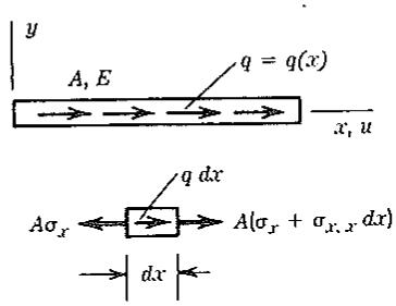Uniform Bar, Axial Load. Equilibrium of axial forces in Fig. 15.4-1 requires that 

text_image

y A, E q = q(x) x, u q dx Aσₓ ← → A(σₓ + σₓ, x dx) dx ←

(a) 

text_image

F_{j-1} \n L \n F_{j-1} \n a \n b \n el.j-1


text_image

Fj L Fj b c el. j

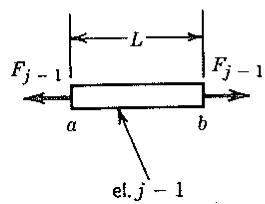
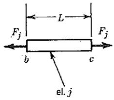
{b} Figure 15.4-1. (a) Uniform elastic bar under distributed axial load q. A = cross-sectional area, E = elastic modulus. (b) Adjacent elements j = .1 and j. Node b is shared after assembly of elements. $A\sigma_{x,x} + q = 0$ . Also, $\sigma_{x} = E\epsilon_{x} = Eu_{,x}$ . Therefore, the governing differential equation in terms of axial displacement u is $$ A E u _ {, x x} + q = 0 \tag {15.4-1} $$ At an end where an axial force $F$ is applied, the nonessential boundary condition is $$ A E u _ {, x} - F = 0 \tag {15.4-2} $$ At a free end, $F = 0$ . Essential boundary conditions consist of prescribed values of $u$ . Let the bar be divided into $\text{numel}$ elements of length $L$ . Each element has the assumed displacement field $$ \bar {u} = \lfloor \mathrm{N} \rfloor \{\mathrm{d} \} \quad \text { where } \quad \left\{ \begin{array}{l} \lfloor \mathrm{N} \rfloor = \left\lfloor \frac {L - x}{L} \frac {x}{L} \right\rfloor \\ \{\mathrm{d} \} = \left\lfloor u _ {1} - u _ {2} \right\rfloor^ {T} \end{array} \right. \tag {15.4-3} $$ and $x = 0$ at the left end of the element. D.o.f. $u_{1}$ and $u_{2}$ are coefficients of modes in the approximating field. Thus $u_{1}$ and $u_{2}$ play the same role as parameters $a_{i}$ in Sections 15.2 and 15.3. Weights $W_{i}$ used in the Galerkin method are therefore $$ W _ {i} = \frac {\partial \bar {u}}{\partial d _ {i}} = N _ {i} \quad \text { where } \quad \left\{ \begin{array}{l} N _ {1} = (L - x) / L \\ N _ {2} = x / L \end{array} \right. \tag {15.4-4} $$ The Galerkin residual equation, Eq. 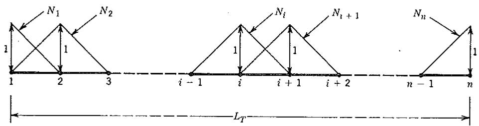15.2-8, becomes $$ \sum_ {j = 1} ^ {\text { numel }} \int_ {0} ^ {L} N _ {i} (A E \bar {u}, _ {x x} + q) d x = 0 \tag {15.4-5} $$ where index i ranges over all shape functions. When elements are assembled, activation of a single d.o.f. activates shape functions in the adjacent elements; that is, linear ramps are activated in elements on either side of the node. Thus, on the structural level, shape functions for all but the first and last nodes are “hat functions,” as shown in Fig. 15.4-2. We see that there are as many structural shape functions as there are d.o.f., and therefore as many Galerkin residual equations as there are d.o.f. If AE is constant, $^{2}$ integration by parts yields $$ \int_ {0} ^ {L} N _ {i} A E \bar {u} _ {, x x} d x = \left[ N _ {i} A E \bar {u} _ {, x} \right] _ {0} ^ {L} - \int_ {0} ^ {L} N _ {i, x} A E \bar {u} _ {, x} d x \tag {15.4-6} $$ From Eq. 15.4-2, the nonessential boundary condition is $AE\bar{u}_{,x} = F$ at element ends. Substituting this and Eq. 15.4-6 into Eq. 15.4-5, we obtain $$ \sum_ {j = 1} ^ {\text {numel}} \int_ {0} ^ {L} \left(- N _ {i, x} A E \bar {u}, _ {x} + N _ {i} q\right) d x + \sum_ {j = 1} ^ {\text {numel}} \left[ N _ {i} F \right] _ {0} ^ {L} = 0 \tag {15.4-7} $$ We adopt the notation $$ \lfloor \mathbf {B} \rfloor = \lfloor \mathbf {N} _ {, x} \rfloor ; \quad \text { then } \quad \bar {u} _ {, x} = \lfloor \mathbf {B} \rfloor \{\mathbf {d} \} = \left\lfloor - \frac {1}{L} \quad \frac {1}{L} \right\rfloor \left\{ \begin{array}{l} u _ {1} \\ u _ {2} \end{array} \right\} \tag {15.4-8} $$ After rearrangement, Eq. 15.4-7 becomes $$ \sum_ {j = 1} ^ {\text {numel}} \underbrace {\int_ {0} ^ {L} \left\lfloor \mathbf {B} \right] ^ {T} A E \left\lfloor \mathbf {B} \right\rfloor d x} _ {[ \mathbf {k} ] _ {j}} \{\mathbf {d} \} = \sum_ {j = 1} ^ {\text {numel}} \underbrace {\int_ {0} ^ {L} \left\lfloor \mathbf {N} \right] ^ {T} q d x} _ {\left\{\mathbf {r} _ {e} \right\} _ {j}} + \sum_ {j = 1} ^ {\text {numel}} \left[ \left\lfloor \mathbf {N} \right] ^ {T} F \right] _ {0} ^ {L} \tag {15.4-9} $$ Except for the last summation, Eq. 15.4-9 clearly yields the standard formula $[\mathbf{K}]\{\mathbf{D}\} = \{\mathbf{R}\}$ , that is, $$ \left(\sum_ {j = 1} ^ {\text { numel }} [ \mathbf {k} ] _ {j}\right) \{\mathbf {D} \} = \sum_ {j = 1} ^ {\text { numel }} \{\mathbf {r} _ {e} \} _ {j} + \{\mathbf {P} \} \tag {15.4-10} $$ where $\{D\}$ replaces $\{d\}$ because of the usual expansion of element matrices to “structure size.” We must explain how the last summation in Eq. 15.4-9 can be regarded as $\{\mathbf{P}\}$ , 

text_image

N₁ N₂ 1 1 1 1 2 3 i - 1 i i + 1 i + 2 N₁ N₁ + 1 1 1 1 n - 1 n Lₜ

Figure 15.4-2. Shape functions active on the structural level after bar elements have been assembled. The number of d.o.f., and shape functions, is $n = \text{numel} + 1$ . the vector of externally applied concentrated loads. At ends of a typical element, x = 0 and x = L, respectively, $$ \left\lfloor \mathrm{N} \right\rfloor_ {0} = \left\lfloor 1 \quad 0 \right] \quad \text { and } \quad \left\lfloor \mathrm{N} \right\rfloor_ {L} = \left\lfloor 0 \quad 1 \right\rfloor \tag {15.4-11} $$ For two adjacent elements $j - 1$ and $j$ , Fig. 15.4-1b, the last summation in Eq. 15.4-9 produces the terms $$ \begin{array}{l} \text {node a} - - - - - - - - - - - - - - - - - - - - - - - - - - - - - - - - - - - - - - - - - - - - - - - - - - - - - - - - - - - - - - - - - - - - - - - - - - - - - - - - - - - - - - - - - - - - - - - - - - - - \\ \text {node b} - - - - - - - - - - - - - - - - - - - - - - - - - - - - - - - - - - - - - - - - - - - - - - - - - - - - - - - - - - - - - - - - - - - - - - - - - - - - - - - - - - - - - - - - - - - - - - - - - - \\ - - - - - - - - - - - - - - - - - - - - - - - - - - - - - - - - - - - - - - - - - - - - - - - - - - - - - - - - - - - - - - - - - - - - - - - - - - - - - - - - - - - - - - - - - - - - - - - - - - - \end{array} + \left( \begin{array}{c} \left\{ \begin{array}{l} 0 \\ 1 \end{array} \right\} F _ {j - 1} \\ - - - - - - - - - - - - - - - - - - - - - - - - - - - - - - - - - - - - - - - - - - - - - - - - - - - - - - - - - - - - - - - - - - - - - - - - - - - - - - - - - - - - - - - - - - - - - - - - - - \left\{ \begin{array}{l} 1 \\ 0 \end{array} \right\} F _ {j} \end{array} \right) + \left\{ \begin{array}{l} 0 \\ 1 \end{array} \right\} F _ {j} \tag {15.4-12} $$ When elements are assembled, as at node $b$ , the resultant axial force $F_{j-1} - F_j$ is produced. This resultant appears in parentheses in Eq. 15.4-12 and is identified as the externally applied load $P$ at node $b$ . Of course, $P$ may be zero; then $F_{j-1} = F_j$ . For the problem of Fig. 15.3-1, load vector $\{\mathbf{P}\}$ would contain only one nonzero entry—namely, $F = \sigma_0 A$ associated with the rightmost node. (Expression 15.4-12 is not used in actual computation; it serves only to explain the transition from Eq. 15.4-9 to Eq. 15.4-10.) Beam Dynamics. In the following example we omit most of the summation signs that indicate assembly of elements and also omit the detailed explanation of nodal loads (as in Eq. 15.4-12). Thus we emphasize the generation of element matrices by the Galerkin method. With $\rho$ the mass density, the mass per unit length is $\rho_{L} = \rho A$ , where $A$ is the cross-sectional area of the beam. The moment-curvature relation is $EIw_{,xx} = M$ . Also, $M_{,x} = V$ and $V_{,x} = q$ , where $EI =$ bending stiffness, $w =$ lateral displacement, $M =$ bending moment, $V =$ transverse shear force, and $q =$ transverse load per unit length. The effective inertia load is $q = -\rho_{L}\ddot{w}$ , where $(^{\prime}) = d() / dt$ . Putting all this together, we obtain the governing differential equation $$ E I w _ {, x x x x} + \rho_ {L} \ddot {w} = 0 \tag {15.4-13} $$ Nonessential boundary conditions are $$ E I w _ {, x x} - M _ {B} = 0 \quad \text { and } \quad E I w _ {, x x x} - V _ {B} = 0 \tag {15.4-14} $$ where $M_{B}$ and $V_{B}$ are prescribed values of bending moment and transverse shear force at ends of the beam. Essential boundary conditions consist of prescribed values of w and $w_{,x}$ . The assumed lateral-displacement field $\tilde{w} = \tilde{w}(x)$ and weight functions $W_{i} = W_{i}(x)$ are given by $$ \bar {w} = \lfloor \mathbf {N} \rfloor \{\mathbf {d} \} \quad \text { and } \quad W _ {i} = N _ {i} \tag {15.4-15} $$ where $\{d\} = \left[w_{1} \quad \theta_{1} \quad w_{2} \quad \theta_{2}\right]^{T}$ and the $N_{i}$ are the usual cubic shape functions (see Fig. 3.13-2). The Galerkin residual equation for a single element is $$ \int_ {0} ^ {L} \left[ \mathbf {N} \right] ^ {T} \left(E I \tilde {w}, _ {x x x x} + \rho_ {L} \ddot {\tilde {w}}\right) d x = 0 \tag {15.4-16} $$ where L is the element length. With EI constant, two integrations by parts yield $$ \int_ {0} ^ {L} \left\lfloor \mathrm{N} \right] ^ {T} E I \bar {w} _ {, x x x x} d x = \int_ {0} ^ {L} \left\lfloor \mathrm{N} _ {, x x} \right] ^ {T} E I \bar {w} _ {, x x} d x + \left[ \left\lfloor \mathrm{N} \right] ^ {T} E I \bar {w} _ {, x x x} - \left\lfloor \mathrm{N} _ {, x} \right] ^ {T} E I \bar {w} _ {, x x} \right] _ {0} ^ {L} \tag {15.4-17} $$ Substitution of Eqs. 15.4-14 and 15.4-17 into Eq. 15.4-16 yields $$ \int_ {0} ^ {L} \left(\left\lfloor \mathbf {N} _ {, x x} \right\rfloor^ {T} E I \tilde {w} _ {, x x} + \rho_ {L} \left\lfloor \mathbf {N} \right\rfloor^ {T} \ddot {\tilde {w}}\right) d x + \left[ \left\lfloor \mathbf {N} \right\rfloor^ {T} V _ {B} - \left\lfloor \mathbf {N} _ {, x} \right\rfloor^ {T} M _ {B} \right] _ {0} ^ {L} = 0 \tag {15.4-18} $$ Terms $V_{B}$ and $M_{B}$ become part of the load vector $\{R\}$ . The argument is analogous to that used in Eqs. 15.4-11 and 15.4-12. From Eq. 15.4-15, $$ \ddot {\bar {w}} = \lfloor \mathbf {N} \rfloor \{\ddot {\mathbf {d}} \} \quad \text { and } \quad \bar {w} _ {, x x} = \lfloor \mathbf {B} \rfloor \{\mathbf {d} \}, \quad \text { where } \quad \lfloor \mathbf {B} \rfloor = \lfloor \mathbf {N} _ {, x x} \rfloor \tag {15.4-19} $$ Substituting Eq. 15.4-19 into Eq. 15.4-18 and assembling elements, we obtain $$ \sum_ {j = 1} ^ {\text { numel }} \left(\int_ {0} ^ {L} [ \mathbf {B} ] ^ {T} E I [ \mathbf {B} ] d x \{\mathbf {d} \} + \int_ {0} ^ {L} \rho_ {L} [ \mathbf {N} ] ^ {T} [ \mathbf {N} ] d x \{\ddot {\mathbf {d}} \}\right) = \{\mathbf {R} \} \tag {15.4-20} $$ which is the standard dynamic equation $[K]\{D\} + [M]\{\ddot{D}\} = \{R\}$ , where $[K]$ and $[M]$ are respectively the structure stiffness and mass matrices and $\{R\}$ represents time-varying loads. 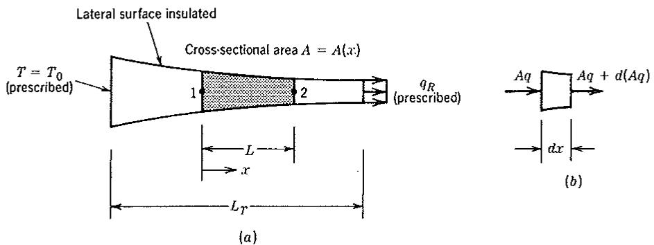Heat Flow in a Bar. We consider steady-state heat conduction in a bar with insulated lateral surface, Fig. 15.4-3a. $^{3}$ Heat flux q is axial and obeys the Fourier heat conduction equation, $q = -kT_{,x}$ . Here k is the thermal conductivity of the material. The negative sign indicates that the direction of heat flow is opposite to the direction of temperature increase. In the steady-state condition, the net rate of heat flow out of a differential element is zero. Thus, from Fig. 15.4-3b, $d(Aq)/dx = 0$ . Combining the two equations $q = -kT_{,x}$ and $d(Aq)/dx = 0$ , we obtain 

text_image

Lateral surface insulated Cross-sectional area A = A(x) T = T₀ (prescribed) 1 2 q_R (prescribed) L x L_T (a) Aq Aq + d(Aq) dx (b)

Figure 15.4-3 (a) Heat flow in a tapered bar. A typical element 1–2 is shown shaded. (b) Heat flow through a differential element. $^{3}$ With J = joule (1 N·m), units of the quantities are T, °C; k, J/m·s·°C; q, J/m $^{2}$ ·s. $$ \frac {d}{d x} (A k T _ {, x}) = 0 \tag {15.4-21} $$ as the governing differential equation. We presume that $Ak$ may vary with $x$ . The approximating temperature field is $\bar{T} = \lfloor \mathbf{N} \rfloor \{\mathbf{T}_e\}$ , where, for a two-node element, nodal temperatures are $\{\mathbf{T}_e\} = \lfloor T_1 - T_2 \rfloor^T$ and the $N_i$ are given by Eq. 15.4-4. Let $q_B$ indicate a boundary heat flux, that is, a heat flux at either end of the element. We write the Galerkin residual equation, integrate by parts, and substitute the nonessential boundary condition $q_B = -k\bar{T}_{,x}$ . Thus $$ \int_ {0} ^ {L} \left\lfloor \mathbf {N} \right] ^ {T} (A k \tilde {T}, _ {x}), _ {x} d x = - \int_ {0} ^ {L} \left\lfloor \mathbf {N}, _ {x} \right] ^ {T} A k \tilde {T}, _ {x} d x - \left[ \left\lfloor \mathbf {N} \right] ^ {T} A q _ {B} \right] _ {0} ^ {L} = 0 \tag {15.4-22} $$ With $\tilde{T}_{,x} = \lfloor \mathbf{N}_{,x}\rfloor \{\mathbf{T}_e\}$ , the element equation becomes $$ \int_ {0} ^ {L} \left\lfloor \mathbf {N}, _ {x} \right\rfloor^ {T} A k \left\lfloor \mathbf {N}, _ {x} \right\rfloor d x \left\{\mathbf {T} _ {e} \right\} = - \left\{ \begin{array}{l} 0 \\ 1 \end{array} \right\} A _ {2} q _ {2 r} + \left\{ \begin{array}{l} 1 \\ 0 \end{array} \right\} A _ {1} q _ {1 r} = \left\{ \begin{array}{c} A _ {1} q _ {1 r} \\ - A _ {2} q _ {2 r} \end{array} \right\} \tag {15.4-23} $$ where $A_{1}q_{1r}$ and $A_{2}q_{2r}$ are respectively heat flow rates at nodes 1 and 2 of the element, each considered positive when heat flows to the right. At the left end of the bar in Fig. 15.4-3a, nodal temperature $T_{0}$ is prescribed instead of a flux $q_{0}$ . It is convenient to adopt the convention that boundary heat flux is considered positive when heat flows into the bar. $^{4}$ Using $q_{1}$ and $q_{2}$ to represent these fluxes, we have $q_{1} = q_{1r}$ and $q_{2} = -q_{2r}$ . Accordingly, for a two-node element in which A and k are constant, Eq. 15.4-23 becomes $$ \frac {A k}{L} \left[ \begin{array}{c c} 1 & - 1 \\ - 1 & 1 \end{array} \right] \left\{ \begin{array}{l} T _ {1} \\ T _ {2} \end{array} \right\} = \left\{ \begin{array}{l} A q _ {1} \\ A q _ {2} \end{array} \right\} \tag {15.4-24} $$ If this uniform element models the entire bar in Fig. 15.4-3a, then $T_{1} = T_{0}$ and $q_{2} = -q_{R}$ , where the negative sign indicates an 'outward flux. Thus Eq. 15.4-24 yields $T_{2} = T_{0} - q_{R}L/k$ and $q_{1} = q_{R}$ . If the boundary conditions were reversed, so that $T_{2} = T_{R}$ is prescribed at the right end and inward flux $q_{1} = q_{0}$ is prescribed at the left end, we would obtain $T_{1} = T_{R} + q_{0}L/k$ and $q_{2} = q_{0}$ . # 15.5 INTEGRATION BY PARTS Integral or “weak” formulations make frequent use of integration by parts. Some useful formulas are now reviewed. Let i, j, and k be unit vectors in the coordinate directions. Also let $F_{1}$ , $F_{2}$ , and $F_{3}$ be independent functions of the coordinates, and $$ \mathbf {F} = F _ {1} \mathbf {i} + F _ {2} \mathbf {j} + F _ {3} \mathbf {k} \quad \text { and } \quad \nu = \ell \mathbf {i} + m \mathbf {j} + n \mathbf {k} \tag {15.5-1} $$ where function F is defined in a volume V, $\nu$ is a unit outward normal on the $^{4}$ This rule is generalized to multidimensional problems by the convention that boundary flux is considered positive in the direction of the inward surface normal vector. surface S of V, and $\ell$ , m, and n are direction cosines of v. The divergence theorem states that $$ \int_ {V} \nabla \cdot \mathbf {F} d V = \int_ {S} \mathbf {F} \cdot \boldsymbol {\nu} d S \tag {15.5-2} $$ where $\nabla \cdot \mathbf{F}$ is the divergence of $\mathbf{F}$ , for example, rectangular coordinates: $\nabla \cdot \mathbf{F} = \frac{\partial F_1}{\partial x} +\frac{\partial F_2}{\partial y} +\frac{\partial F_3}{\partial z}$ (15.5-3a) cylindrical coordinates: $\nabla \cdot \mathbf{F} = \frac{1}{r} \frac{\partial}{\partial r} (rF_1) + \frac{1}{r} \frac{\partial F_2}{\partial \theta} + \frac{\partial F_3}{\partial z}$ (15.5-3b) In Eq. 15.5-2, F and its first partial derivatives must be continuous in V and on S, and integration must proceed over all boundaries, interior as well as exterior. Let $P$ and $Q$ be functions of the coordinates. Then, for example, $(PQ)_{,x} = P_{,x}Q + PQ_{,x}$ . Therefore $$ \int_ {V} P Q _ {, x} d V = - \int_ {V} P _ {, x} Q d V + \int_ {V} (P Q) _ {, x} d V \tag {15.5-4} $$ If we regard $PQ$ as $F_{1}$ in Eq. 15.5-3a and let $F_{2} = F_{3} = 0$ , Eq. 15.5-2 allows us to replace the last integral in Eq. 15.5-4 by a surface integral. Thus Eq. 15.5-4 becomes the following formula for integration by parts in rectangular coordinates: $$ \int_ {V} P Q _ {, x} d V = - \int_ {V} P _ {, x} Q d V + \int_ {S} P Q \ell d S \tag {15.5-5} $$ Analogous formulas for the $x$ and $y$ derivatives are easy to derive. The same procedure may be applied in cylindrical coordinates. For example, $$ \int_ {V} \frac {1}{r} \frac {\partial}{\partial r} (r P Q) d V = \int_ {V} \left[ \frac {\partial P}{\partial r} Q + P \frac {1}{r} \frac {\partial}{\partial r} (r Q) \right] d V \tag {15.5-6} $$ We let $F_{1} = PQ$ and $F_{2} = F_{3} = 0$ in Eq. 15.5-3b, solve for the last term in Eq. 15.5-6, and apply Eq. 15.5-2. Thus $$ \int_ {V} P \frac {1}{r} \frac {\partial}{\partial r} (r Q) d V = - \int_ {V} \frac {\partial P}{\partial r} Q d V + \int_ {S} P Q \ell d S \tag {15.5-7} $$ In similar fashion, $$ \int_ {V} \frac {1}{r} P \frac {\partial Q}{\partial \theta} d V = - \int_ {V} \frac {1}{r} \frac {\partial P}{\partial \theta} Q d V + \int_ {S} P Q m d S \tag {15.5-8} $$ Formulas for integration by parts in two dimensions can be obtained directly from the preceding formulas by setting $F_{3} = 0$ in Eqs. 15.5-3 and presuming that integration with respect to z has already been done across a unit thickness. # 15.6 TWO-DIMENSIONAL PROBLEMS The Quasiharmonic Equation. The “quasiharmonic” equation describes heat conduction and various other physical problems, as explained in more detail in Chapter 16. Here, without specifying the physical problem, we illustrate the formulation of element matrices by the Galerkin method. Consider a plane region of unit thickness, volume V, and boundary S. The governing equation and the nonessential boundary condition are, respectively, $$ \text { in } V, \frac {\partial}{\partial x} (k _ {x} \phi_ {, x}) + \frac {\partial}{\partial y} (k _ {y} \phi_ {, y}) + Q = 0 \tag {15.6-1} $$ $$ \text { on } S, \quad \ell k _ {x} \phi_ {, x} + m k _ {y} \phi_ {, y} - q _ {B} = 0 \tag {15.6-2} $$ where $\phi = \phi(x, y)$ is the dependent variable and $\ell$ and $m$ are direction cosines of an outward normal to $S$ . Known quantities $k_x, k_y$ , and $Q$ may be either constant or functions of $x$ and $y$ . In the nonessential boundary condition, $q_B$ is a prescribed boundary flux, positive when directed into $V$ . Essential boundary conditions, which in general prevail over only a portion of $S$ , consist of prescribed values of $\phi$ . For the special case $k_x = k_y = \text{constant}$ and $Q = 0$ , Eq. 15.6-1 becomes Laplace's equation $\nabla^2\phi = 0$ . A function $\phi$ that satisfies $\nabla^2\phi = 0$ is called harmonic. The approximating field $\tilde{\phi}$ is $$ \tilde {\phi} = \lfloor \mathbf {N} \rfloor \{\phi_ {e} \} = \left\lfloor N _ {1} \quad N _ {2} \quad \dots \quad N _ {n} \right\rfloor \{\phi_ {e} \} \tag {15.6-3} $$ where n is the number of nodes per element and $\{\phi_{e}\}$ is the vector of element nodal d.o.f. The Galerkin residual equation is $$ \iint [ \mathbf {N} ] ^ {T} \left[ \frac {\partial}{\partial x} \left(k _ {x} \bar {\phi}, _ {x}\right) + \frac {\partial}{\partial y} \left(k _ {y} \bar {\phi}, _ {y}\right) + Q \right] d x d y = 0 \tag {15.6-4} $$ Integration by parts (e.g., Eq. 15.5-5) yields $$ \iint \left\lfloor \mathrm{N} \right] ^ {T} \frac {\partial}{\partial x} \left(k _ {x} \tilde {\phi} _ {, x}\right) d x d y = - \iint \left\lfloor \mathrm{N} _ {, x} \right] ^ {T} k _ {x} \tilde {\phi} _ {, x} d x d y + \int \left\lfloor \mathrm{N} \right] ^ {T} k _ {x} \tilde {\phi} _ {, x} \ell d S \tag {15.6-5a} $$ $$ \int \int \left\lfloor \mathbf {N} \right] ^ {T} \frac {\partial}{\partial y} \left(k _ {y} \bar {\phi} _ {, y}\right) d x d y = - \int \int \left\lfloor \mathbf {N} _ {, y} \right] ^ {T} k _ {y} \bar {\phi} _ {, y} d x d y + \int \left\lfloor \mathbf {N} \right] ^ {T} k _ {y} \bar {\phi} _ {, y} m d S \tag {15.6-5b} $$ Substitution of Eqs. 15.6-5 and 15.6-2 into Eq. 15.6-4 yields $$ \iint \left(- \left\lfloor \mathrm{N}, _ {x} \right] ^ {T} k _ {x} \tilde {\phi}, _ {x} - \left\lfloor \mathrm{N}, _ {y} \right] ^ {T} k _ {y} \tilde {\phi}, _ {y} + \left\lfloor \mathrm{N} \right] ^ {T} Q\right) d x d y + \int \left\lfloor \mathrm{N} \right] ^ {T} q _ {B} d S = 0 \tag {15.6-6} $$ Finally, substitution of $\tilde{\phi}_{,x} = \lfloor \mathbf{N}_{,x}\rfloor \{\phi_e\}$ and $\tilde{\phi}_{,y} = \lfloor \mathbf{N}_{,y}\rfloor \{\phi_e\}$ into Eq. 15.6-6 yields $$ \begin{array}{l} \left[ \iint \left(\lfloor \mathrm{N}, _ {x} \rfloor^ {T} k _ {x} \lfloor \mathrm{N}, _ {x} \rfloor + \lfloor \mathrm{N}, _ {y} \rfloor^ {T} k _ {y} \lfloor \mathrm{N}, _ {y} \rfloor\right) d x d y \right] \left\{\phi_ {e} \right\} \\ = \iint \left\lfloor \mathbf {N} \right] ^ {T} Q d x d y + \int \left\lfloor \mathbf {N} \right] ^ {T} q _ {B} d S \tag {15.6-7} \\ \end{array} $$ Or, in customary notation, $[\mathbf{k}]\{\phi_e\} = \{\mathbf{r}\}$ . Plane Elasticity. The foregoing manipulations are little changed in application to problems of plane stress or plane strain. We summarize as follows. The governing differential equations are the equilibrium equations, and the nonessential boundary conditions involve boundary tractions $\Phi_{x}$ and $\Phi_{y}$ , that is, $$ \sigma_ {x, x} + \tau_ {x y, y} + F _ {x} = 0 \quad \text { and } \quad \ell \sigma_ {x} + m \tau_ {x y} = \Phi_ {x} \tag {15.6-8} $$ $$ \tau_ {x y, x} + \sigma_ {y, y} + F _ {y} = 0 \quad \ell \tau_ {x y} + m \sigma_ {y} = \Phi_ {y} $$ where $F_{x}$ and $F_{y}$ are body forces per unit volume, and $\ell$ and m are direction cosines of an outward normal to the boundary. Essential boundary conditions consist of prescribed values of displacements u and v. The element displacement field is $$ \{\tilde {\mathbf {u}} \} = \left\{ \begin{array}{l} \tilde {u} \\ \tilde {v} \end{array} \right\} = \left[ \begin{array}{l l} \lfloor \mathbf {N} \rfloor & \lfloor \mathbf {0} \rfloor \\ \lfloor \mathbf {0} \rfloor & \lfloor \mathbf {N} \rfloor \end{array} \right] \{\mathbf {d} \} \tag {15.6-9} $$ where $\{\mathbf{d}\} = \lfloor u_1 \quad u_2 \quad \ldots \quad u_n \quad v_1 \quad v_2 \quad \ldots \quad v_n \rfloor^T$ and $\lfloor \mathbf{N} \rfloor = \lfloor N_1 \quad N_2 \quad \ldots \quad N_n \rfloor$ for an $n$ -node element (e.g., Eqs. 3.12-10 for a four-node rectangle). The arrangement of terms in Eq. 15.6-9 is adopted only for convenience of notation. As there are now two differential equations, there are two Galerkin residual equations, that is, $$ \begin{array}{l} \iint \left\lfloor \mathbf {N} \right] ^ {T} \left(\tilde {\sigma} _ {x, x} + \tilde {\tau} _ {x y, y} + F _ {x}\right) d x d y = 0 \\ \text { and } \quad \cdot \int \int \left[ \mathbf {N} \right] ^ {T} (\tilde {\tau} _ {x y, x} + \tilde {\sigma} _ {y, y} + F _ {y}) d x d y = 0 \tag {15.6-10} \\ \end{array} $$ where $\bar{\sigma}_{x}$ , $\bar{\sigma}_{y}$ , and $\bar{\tau}_{xy}$ are the approximate stress fields produced by Eq. 15.6-9, the strain–displacement relations, and the stress–strain relations. There are four terms in Eqs. 15.6-10 to be integrated by parts. For example, the first such integration yields $$ \iint \left\lfloor \mathbf {N} \right\rfloor^ {T} \tilde {\sigma} _ {x, x} d x d y = - \iint \left\lfloor \mathbf {N}, _ {x} \right\rfloor^ {T} \tilde {\sigma} _ {x} d x d y + \int \left\lfloor \mathbf {N} \right\rfloor^ {T} \tilde {\sigma} _ {x} \ell d S \tag {15.6-11} $$ By this process the nonessential boundary conditions are introduced. Next, we introduce the relations $$ \{\boldsymbol {\sigma} \} = [ \mathrm{E} ] (\{\boldsymbol {\epsilon} \} - \{\boldsymbol {\epsilon} _ {0} \}) + \{\boldsymbol {\sigma} _ {0} \} \tag {15.6-12} $$ $$ \{\epsilon \} = [ \partial ] \{\bar {\mathbf {u}} \} = [ \mathbf {B} ] \{\mathbf {d} \} \tag {15.6-13} $$ where $[\partial]$ is the differential operator defined in Eq. 1.5-6. The final result given by Eqs. 15.6-10 is the same as given by Eqs. 4.1-5 and 4.1-6. # PROBLEMS # Section 15.3 15.1 Derive the differential equation shown in Fig. 15.3-1. 15.2 Verify that despite collocation at $x = L_{T} / 3$ , Eqs. 15.3-2 and 15.3-4 do not yield $\bar{u} = u$ at $x = L_{T} / 3$ . Does this indicate that something is wrong? Explain. 15.3 Show that the Galerkin condition $R_{i} = 0$ in Eq. 15.3-13 is the same as the stationary-functional condition $\partial \Pi / \partial a_{i} = 0$ if functional $\Pi$ is given by $$ \Pi = \int_ {0} ^ {L _ {T}} \left(\frac {1}{2} \tilde {u} _ {, x} ^ {2} - c x \tilde {u}\right) d x - [ b \tilde {u} ] _ {x = L _ {T}} $$ 15.4 Consider the differential equation $u_{,xx} + 4u = 12$ , with essential boundary conditions $u = 3$ at $x = 0$ and $u = 1$ at $x = 1$ . There are no nonessential boundary conditions. The exact solution is $u = 3 - 2.1995 \sin 2x$ . A one-parameter approximating polynomial that meets the essential boundary conditions is $\bar{u} = 3 - 2x + a(x^2 - x)$ . Determine parameter $a$ in the range $0 < x < 1$ by (a) collocation, (b) subdomain, (c) least squares, (d) least squares collocation, and (e) Galerkin methods. Choose points at $x = 0.5$ in part (a) and at $x = \frac{1}{3}$ and $x = \frac{2}{3}$ in part (d). In each case calculate the percentage error of $\bar{u}$ at $x = 0.5$ and at $x = 0.7$ . 15.5 Consider the differential equation $u_{,x} + 2u - 16x = 0$ with the boundary condition $u = 0$ at $x = 0$ . The exact solution is $u = 4(e^{-2x} - 1) + 8x$ . A two-parameter approximating polynomial that satisfies the boundary condition is $\tilde{u} = a_1x + a_2x^2$ . Determine $a_1$ and $a_2$ in the range $0 < x < 1$ and compute percentage errors of $\tilde{u}$ at $x = 0.5$ and at $x = 0.7$ . (a) Use least-squares collocation, with collocation points at $x = 0.25$ , $x = 0.50$ , and $x = 0.75$ . (b) Use the Galerkin method. 15.6 Solve the problem defined by Eq. 15.3-1 in each of the following ways. Compare your answers with those in Table 15.3-1. (a) Use collocation, with the sampling point at $x = L_T / 2$ . (b) Use subdomain and integrate over the span $0 \leq x \leq L_T / 2$ . (c) Use least squares collocation. Evaluate $R_{D}$ at $x = 0$ , $x = L_{T} / 2$ , and $x = L_{T}$ . Use $\alpha = 1 / L_{T}$ . (d) Omit the residual $R_{D2}$ in Eq. 15.3-7. (e) Show why, in this particular problem, the solution provided by least squares collocation is independent of $\alpha$ . 15.7 In Fig. 15.3-1, let $\sigma_0 = 0$ and let $q$ be the uniform traction $q = q_0$ , but acting on the right half $L_T / 2 < x < L_T$ only. As in Section 15.3, determine two-parameter approximate solutions by the five methods illustrated. In collocation, choose the point $x = 2L_T / 3$ ; otherwise, proceed as in Section 15.3. Compare exact and approximate results for the case $q_0 = L_T = AE = 1$ . 15.8 Consider a uniform, simply supported beam of length L. For each of the following loadings, use the Galerkin method to determine constant a in the approximating lateral displacement field $\bar{w} = ax(L - x)$ . Also compute the percentage error of the predicted midspan deflection.