text_image
σ
σγ
E
D
εγ
A
B
E
C
ε
εp
εe = σB/E
dεp
dεe
dε
(a)
text_image
σ
σB
σY
B
E
E
2σY
|σB - 2σY|
Ei
Ei
σB
Kinematic
Isotropic
-σ
{b}
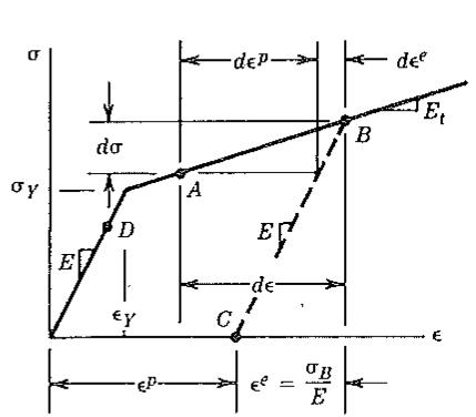
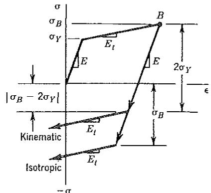
Figure 17.3-1. (a) Stress-strain plot in uniaxial stress, idealized as two straight lines, where $\sigma_{Y}$ is the stress at first onset of yielding. (b) Kinematic and isotropic hardening rules.
$$
d \sigma = E (d \epsilon - d \epsilon^ {p}) \quad d \sigma = E _ {t} d \epsilon \quad \text { and } \quad d \sigma = H d \epsilon^ {p} \tag {17.3-1}
$$
where H is called the strain-hardening parameter. Substitution of the first and third of Eqs. 17.3-1 into the second yields
$$
H = \frac {E _ {t}}{1 - (E _ {t} / E)} \quad \text { or } \quad E _ {t} = E \left(1 - \frac {E}{E + H}\right) \tag {17.3-2}
$$
where $E_{t}$ is the tangent modulus. When written in this form, the expression for $E_{t}$ is similar to a more general expression used for multiaxial states of stress. If E is finite and $E_{t} = 0$ , then H = 0, and the material is called “elastic–perfectly plastic.”
A summary of elastic–plastic action in uniaxial stress is as follows. The yield criterion states that yielding begins when $|\sigma|$ reaches $\sigma_{Y}$ , where in practice $\sigma_{Y}$ is usually taken as the tensile yield strength. Subsequent plastic deformation may alter the stress needed to produce renewed or continued yielding; this stress exceeds the initial yield strength $\sigma_{Y}$ if $E_{t} > 0$ . A flow rule can be written in multidimensional problems. It leads to a relation between stress increments $\{d\sigma\}$ and strain increments $\{d\epsilon\}$ . In uniaxial stress this relation is simply $d\sigma = E_{t} d\epsilon$ , which describes the increment of stress produced by an increment of strain. Note, however, that if the material has yet to yield or is unloading, then $d\sigma = E d\epsilon$ (e.g., in Fig. 17.3-1a, complete unloading from point B leads to point C and a permanent strain $e^{p}$ ). Finally, there is a hardening rule, which describes how the yield criterion is changed by the history of plastic flow. For example, imagine that unloading occurs from point B in Fig. 17.3-1a. With reloading from point C, response will be elastic until $\sigma > \sigma_{B}$ , when renewed yielding occurs. If we assume that yielding reappears when $|\sigma| > \sigma_{B}$ , whether $\sigma$ is tensile or compressive, we have adopted the “isotropic hardening” rule (Fig. 17.3-1b). However, for common metals, such a rule is in conflict with the observed behavior that yielding reappears at a stress of approximate magnitude $\sigma_{B} - 2\sigma_{Y}$ when loading is reversed. Accordingly, a better match to observed behavior is provided by the “kinematic hardening” rule, which (for uniaxial stress) says that a total elastic range of $2\sigma_{Y}$ is preserved.
The discussion in the foregoing paragraph does not require that postelastic response be idealized as a straight line. In other words, $E_{t}$ need not be constant.
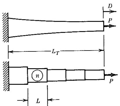
As a simple application of one-dimensional plasticity, imagine that a tapered bar is to be loaded by an axial force $P$ (Fig. 17.3-2). Material properties are those depicted in Fig. 17.3-1. The bar is modeled by two-d.o.f. bar elements, each of constant cross section. For elastic conditions, the element stiffness matrix is given by Eq. 2.4-5, where $E = d\sigma / d\epsilon$ when $|\sigma| < \sigma_{Y}$ . Upon yielding, the stress-strain relation becomes $E_{t} = d\sigma / d\epsilon$ . Accordingly, letting $E_{\mathrm{ep}}$ represent the "elastic-plastic" stiffness, we write the element tangent-stiffness matrix as
$$
[ \mathbf {k} _ {t} ] = \frac {A E _ {\mathrm{ep}}}{L} \left[ \begin{array}{c c} 1 & - 1 \\ - 1 & 1 \end{array} \right] \tag {17.3-3}
$$
where $E_{\mathrm{ep}} = E$ if the yield criterion is not exceeded or if unloading is taking place, and $E_{\mathrm{ep}} = E_t$ if plastic flow is involved.
In numerical solutions, material may make the transition from elastic to plastic within an iterative cycle of the solution process. For example, imagine that $d\epsilon$ spans $\epsilon_{D}$ to $\epsilon_{A}$ in Fig. 17.3-1a. The problem of “rounding the corner” can be addressed by combining $E$ and $E_{t}$ according to the fraction $m$ of the total step $d\epsilon$ that is elastic. Thus let
$$
E _ {\mathrm{ep}} = m E + (1 - m) E _ {t} \quad \text { where } \quad m = \frac {\epsilon_ {Y} - \epsilon_ {D}}{\epsilon_ {A} - \epsilon_ {D}} \tag {17.3-4}
$$
Alternatively, by substituting stresses for strains and using the fictitious stress $\sigma^{*} = E\epsilon_{A}$ , we can write $m$ in terms of stresses, as $m = (\sigma_{Y} - \sigma_{D}) / (\sigma^{*} - \sigma_{D})$ . Refinements of this scheme are possible [17.11].
The present discussion excludes thermal strains and creep strains. In general, these effects may appear in combination with elastic–plastic action. Then the total strain increment $d\epsilon^{tot}$ is a combination of elastic, plastic, thermal, and creep strain components. The strain increment $d\epsilon = d\epsilon^{e} + d\epsilon^{p}$ used in elastic–plastic analysis excludes thermal and creep strains. Thus
$$
d \epsilon^ {e} + d \epsilon^ {p} = d \epsilon^ {\mathrm{tot}} - d \epsilon^ {T} - d \epsilon^ {C} \tag {17.3-5}
$$
text_image
D
P
L_T
n
P
L
(a)
line
| D | P (Exact) | P (ΔP₁) | P (ΔP₂) | P (ΔP₃) |
|---------|-----------|---------|---------|---------|
| 0 | 0 | 0 | 0 | 0 |
| D₁ | ~0.5 | ~0.5 | ~0.5 | ~0.5 |
| D₂ | ~1.0 | ~1.0 | ~1.0 | ~1.0 |
| D₃ | ~1.5 | ~1.5 | ~1.5 | ~1.5 |
(b)
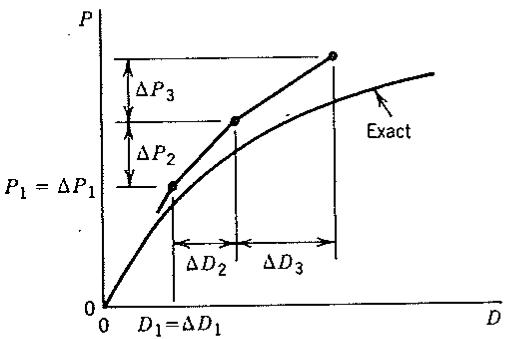
Figure 17.3-2. (a) A tapered bar and a finite element model using uniform elements, of which element n is typical. (b) Progress of a tangent-stiffness solution if step 3 of the algorithm is omitted. D = displacement of load P.
Tangent-Stiffness Method. Consider the tapered bar depicted in Fig. 17.3-2a. It is desired to trace the quasistatic load versus displacement curve and determine element stresses by means of a finite element model and load increments $\Delta P$ . Increments are small but not infinitesimal, so that $d\epsilon$ becomes $\Delta\epsilon$ , and the numerical solution is not exact. A numerical representation of the stress–strain relation must be stored, so that $\sigma$ , E, and $E_{t}$ can be obtained for any $\epsilon$ . The algorithm outlined below requires that we also store, and update after each computational cycle, the nodal displacements $\{D\}$ , element strains $\epsilon$ , and element stresses $\sigma$ . With two-d.o.f. bar elements (Eq. 17.3-3), $\sigma$ and $\epsilon$ are constant over each element length L.
1. For the first computational cycle $(i = 1)$ , assume $E_{\mathfrak{ep}} = E$ for all elements. Apply the first load increment, $\{\Delta \mathbf{R}\}_{1}$ .
2. Using the current strains, determine the current $E_{\mathrm{ep}}$ in each element. Use Eq. 17.3-3 to obtain $[\mathbf{k}_t]_n$ for each element $n$ . Obtain the current structure tangent stiffness $[\mathbf{K}_t]_{i-1} = \hat{\Sigma} [\mathbf{k}_t]_n$ . Solve $[\mathbf{K}_t]_{i-1}\{\Delta \mathbf{D}\}_i = \{\Delta \mathbf{R}\}_i$ for $\{\Delta \mathbf{D}\}_i$ . (For the bar of Fig. 17.3-2a, $\Delta P$ at the right end is the only nonzero entry in $\{\Delta \mathbf{R}\}_i$ .) From $\{\Delta \mathbf{D}\}_i$ , obtain current strain increments $\Delta \epsilon_i$ for each element.
3. Optional. If any elements make the elastic-to-plastic transition, use Eq. 17.3-4 to revise $E_{\mathrm{ep}}$ for each such element, and go back to step 2. Without changing the applied load $\{\Delta \mathbf{R}\}_i$ , repeat steps 2 and 3 until convergence, which may be defined as $\Delta \epsilon$ being less than a prescribed fraction of the accumulated total $\epsilon$ in every element. These operations represent secant-stiffness iterations (see Fig. 17.2-2a) within one of the load steps of the tangent-stiffness procedure.
4. Update: $\{\mathbf{D}\}_{i} = \{\mathbf{D}\}_{i-1} + \{\Delta \mathbf{D}\}_{i}$ , and for each element, $\epsilon_{i} = \epsilon_{i-1} + \Delta \epsilon_{i}$ and $\sigma_{i} = \sigma_{i-1} + \Delta \sigma_{i}$ , where $\Delta \sigma_{i} = (E_{\mathrm{ep}})_{i} \Delta \epsilon_{i}$ . For the first cycle ( $i = 1$ ), initial values (subscript $i - 1$ ) of displacement, strain, and stress are typically all zero if one starts from the unloaded configuration, but are nonzero if one starts from a state in which plastic action impends.
5. Apply the next load increment and return to step 2.
6. Stop when $\Sigma \{\Delta \mathbf{R}\}_{i}$ reaches the total applied load.
Three cycles of the foregoing algorithm are depicted in Fig. 17.3-2b. Each cycle produces a line segment whose slope corresponds to the current stiffness. Drift from the exact path can be reduced by using smaller load increments, by exercising step 3 previously discussed, and by using “corrective loads,” which are discussed in Section 17.5. Step 3 can be avoided by using load increments $\{\Delta R\}_{i}$ that bring a single element to the verge of yielding as each load increment is added. This is easily accomplished by scaling the incremental tangent-stiffness solutions.
The foregoing incremental procedure is essentially a Newton–Raphson method; that is, a new tangent-stiffness matrix is used in each computational cycle.
Initial-Stiffness Method. Again we seek displacements and stresses in a structure in which plastic action occurs. One can apply the iterative method described by Eq. 17.2-3 and Fig. 17.2-2b. Thus the original elastic stiffness matrix is used at all times. The effects of plastic action are regarded as initial stresses that produce fictitious loads, which are combined with the load actually applied (accordingly, this procedure is often called the initial-stress method). This procedure avoids
the expense of repeatedly forming and factoring a tangent-stiffness matrix, but may converge slowly if plastic strains are large or widespread [17.12].
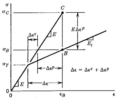
In Fig. 17.3-3a, imagine that we seek the strain $\epsilon_{B}$ associated with stress $\sigma_{B}$ . We can obtain $\epsilon_{B}$ using only the elastic modulus $E$ by writing $\epsilon_{B} = \sigma_{C} / E$ . Here $\sigma_{C}$ is the fictitious stress $\sigma_{C} = \sigma_{B} + E \Delta \epsilon^{p}$ .
In computation, $e^{p}$ can be obtained by accumulating the plastic strain increments $\Delta e^{p}$ produced in the iterative cycles. From Eqs. 17.3-1,
$$
\Delta \epsilon^ {p} = \frac {1}{H} \Delta \sigma = \frac {1}{H} E _ {t} \Delta \epsilon = \frac {E}{E + H} \Delta \epsilon = \left(1 - \frac {E _ {t}}{E}\right) \Delta \epsilon \tag {17.3-6}
$$
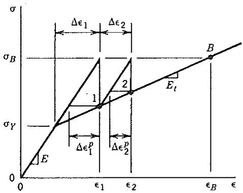
In computation, the progression to $\epsilon_{B}$ is made in a series of steps, as shown in Fig. 17.3-3b, using “supplementary loads” defined in Eq. 17.3-7. It is not necessary that the stress–strain relation be piecewise linear.
The calculation procedure for a structure such as that in Fig. 17.3-2a is as follows.
1. Compute the elastic stiffness matrix [K] (which is identically the initial tangent-stiffness matrix). Solve $[K]\{D\} = \{R\}$ for $\{D\}$ , where $\{R\}$ is proportional to the actual load but of arbitrary level. From this solution, scale $\{R\}$ so that it becomes $\{R_{Y}\}$ , which causes yielding to impend. Scale $\{D\}$ similarly and call the result $\{D\}_{old}$ . Subsequent load increments may be chosen as $\{\Delta R\} = 0.05 \{R_{Y}\}$ or as $\{\Delta R\} = (E_{T}/E)\{R_{Y}\}$ , whichever is greater [17.13]. Initialize supplementary loads $\{\Delta R_{s}\}$ to zero.
2. Solve the equations $[K]\{\Delta D\} = \{\Delta R\} + \{\Delta R_{s}\}$ for $\{\Delta D\}$ .
3. Update displacements: $\{\mathbf{D}\}_{\text{new}} = \{\mathbf{D}\}_{\text{old}} + \{\Delta \mathbf{D}\}$ .
4. In each element, calculate the strain increment $\Delta \epsilon$ associated with $\{\Delta \mathbf{D}\}$ . Update element stress by adding $\Delta \sigma$ to the existing stress $\sigma$ , using $\Delta \sigma = E \Delta \epsilon$ if $\sigma < \sigma_Y$ and $\Delta \sigma = E_t \Delta \epsilon$ if $\sigma > \sigma_Y$ . For elements that make the elastic-to-plastic transition by the addition of $\Delta \sigma$ , evaluate $m$ by Eq. 17.3-4 and recompute $\Delta \sigma$ as $\Delta \sigma = Em \Delta \epsilon$ .
5. For all elements that display plastic strains ( $|\sigma| > \sigma_{Y}$ in Fig. 17.3-3), calculate plastic strain increments according to Eq. 17.3-6. In this calculation, use $(1 - m)\Delta\epsilon$ rather than $\Delta\epsilon$ for elements that make the elastic-to-plastic
line
| Point | ε | σ | Δε |
|-------|-------|-------|--------|
| E | 0 | 0 | Δε^e |
| B | ε_B | 0 | Δε^p |
| C | ε_B | σ_C | Δε^p |
| E_t | ε_B | σ_B | Δε^p |
(a)
line
| Point | ε | σ | Label |
|-------|------|------|-------|
| 1 | ε₁ | σY | E |
| 2 | ε₂ | σY | 1 |
| B | ε_B | σY | B |
(b)
Figure 17.3-3. (a) $E \Delta e^{p}$ is regarded as an initial stress. (b) Iterative approach to the solution point B.
transition (see Eq. 17.3-4). Generate the supplementary loads by summing element contributions:
$$
\left\{\Delta \mathbf {R} _ {s} \right\} = \sum \left\{\Delta \mathbf {r} _ {s} \right\} \quad \text { where } \quad \left\{\Delta \mathbf {r} _ {s} \right\} = \int_ {0} ^ {L} \left\lfloor \mathbf {B} \right] ^ {T} E \Delta e ^ {p} A d x \tag {17.3-7}
$$
Solve the equations $[K]\{\Delta D\} = \{\Delta R_{s}\}$ for $\{\Delta D\}$ . Return to step 3.
6. Repeat steps 3 through 5 until convergence. Then apply another load increment $\{\Delta R\}$ and return to step 2.
7. Stop when $\{R_{Y}\} + \Sigma\{\Delta R\}$ reaches the total applied load.
# 17.4 SMALL-STRAIN PLASTICITY RELATIONS
Multiaxial states of stress can be analyzed if the theory in Section 17.3 is generalized. The following is a summary. In our discussion we use the engineering definition of shear strain (e.g., $\gamma_{xy} = u_{,y} + v_{,x}$ ), not the tensor definition (e.g., $\epsilon_{xy} = (u_{,y} + v_{,x})/2$ ).
General. Plasticity theory has three parts: a yield criterion, a flow rule, and a hardening rule. The general theory and its various special forms are contrived to fit experimental data.
Yield Criterion. We define a yield function F, which is a function of stresses $\{\sigma\}$ and quantities $\{\alpha\}$ and $W_{p}$ associated with the hardening rule. Yielding occurs when
$$
F (\sigma , \alpha , W _ {p}) = 0 \tag {17.4-1}
$$
where $\{\alpha\}$ and $W_{p}$ are defined by Eq. 17.4-3. Specifically, if we evaluate F using given values of $\{\sigma\}$ , $\{\alpha\}$ , and $W_{p}$ , then the possible results are F < 0 and F = 0. Respectively, these results mean that the material is in the elastic range or is yielding. The result F > 0 is not physically possible, as it indicates a state of stress that does not satisfy the constitutive law (e.g., $\sigma_{C}$ in Fig. 17.3-3 is not physically possible). Similarly, the respective results dF < 0 and dF = 0 imply elastic unloading and continued yielding. The result dF > 0 is not possible in the plastic regime.
Flow Rule. We define a plastic potential Q, which has units of stress and is a function of the stresses, $Q = Q(\sigma, \alpha, W_{p})$ . With $d\lambda$ a scalar that may be called a “plastic multiplier,” plastic strain increments are given by
$$
\left\{d \epsilon^ {p} \right\} = \left\{\frac {\partial Q}{\partial \sigma} \right\} d \lambda \tag {17.4-2}
$$
Thus $de_{x}^{e} = (\partial Q/\partial \sigma_{x}) \, d\lambda$ , and so on. The flow rule is called “associated” if Q = F and “nonassociated” otherwise. Associated flow rules are commonly used for ductile metals, but nonassociated rules are better suited to soil and granular materials.
Hardening Rule. In Eq. 17.4-1, $\{\alpha\}$ locates the center of the yield surface in stress space. Initially, before any plastic strains appear, $\{\alpha\} = \{0\}$ . In “kinematic hardening,” the center moves in the direction of plastic straining, so that $\{\alpha\}$ becomes nonzero. Parameter $W_{p}$ describes how the yield surface grows. In “isotropic hardening,” $W_{p}$ is nonzero but $\{\alpha\}$ is zero. Quantities $\{\alpha\}$ and $W_{p}$ are defined as
$$
\{\boldsymbol {\alpha} \} = \int C \left\{d \boldsymbol {\epsilon} ^ {p} \right\} \quad \text { and } \quad W _ {p} = \int \left\{\boldsymbol {\sigma} \right\} ^ {T} \left\{d \boldsymbol {\epsilon} ^ {p} \right\} \tag {17.4-3}
$$
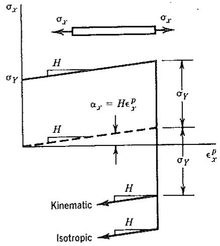
where C can be assumed to be a material constant [17.13,17.14]. For purely kinematic hardening, C = H (Fig. 17.4-1). $W_{p}$ can be identified as plastic work per unit volume. (Use of $W_{p}$ in F implies a “work-hardening” model. Alternatively, $W_{p}$ can be replaced by an effective plastic strain $\epsilon_{ef}^{p}$ , which implies a “strain-hardening” model. Either model can be used to represent isotropic hardening.)
An incremental stress–strain relation, analogous to the relation $\{\sigma\} = [E]\{\epsilon\}$ of elasticity but valid into the elastic–plastic regime, can be derived as follows. First, we differentiate Eq. 17.4-1:
$$
d F = 0 = \left\{\frac {\partial F}{\partial \sigma} \right\} ^ {T} \{d \sigma \} + \left\{\frac {\partial F}{\partial \alpha} \right\} ^ {T} \{d \alpha \} + \frac {\partial F}{\partial W _ {p}} d W _ {p} \tag {17.4-4}
$$
From Eqs. 17.4-3 we obtain $\{d\alpha\} = C\{d\epsilon^{p}\}$ and $dW_{p} = \{\sigma\}^{T}\{d\epsilon^{p}\}$ . In addition, in multidimensional analogy to Eq. 17.3-1, we have
$$
\{d \sigma \} = [ \mathbf {E} ] \{d \epsilon^ {e} \} = [ \mathbf {E} ] (\{d \epsilon \} - \{d \epsilon^ {p} \}) \tag {17.4-5}
$$
where $\{d\epsilon\}$ is assumed to contain no creep or thermal strains (see Eq. 17.3-5). Making these substitutions into Eq. 17.4-4, using Eq. 17.4-2 to eliminate $\{d\epsilon^{p}\}$ , and solving for the plastic multiplier $d\lambda$ , we obtain
$$
d \lambda = \{\mathbf {C} _ {\lambda} \} ^ {T} \{d \epsilon \} \tag {17.4-6}
$$
text_image
σₓ
σᵧ
H
αₓ = Hεₓᵖ
H
σᵧ
σᵧ
εₓᵖ
Kinematic
H
Isotropic
H
Figure 17.4-1. Stress versus plastic strain in uniaxial stress.
where
$$
\left\{\mathbf {C} _ {\lambda} \right\} ^ {T} = \frac {\left\{\frac {\partial F}{\partial \boldsymbol {\sigma}} \right\} ^ {T} [ \mathbf {E} ]}{\left\{\frac {\partial F}{\partial \boldsymbol {\sigma}} \right\} ^ {T} [ \mathbf {E} ] \left\{\frac {\partial Q}{\partial \boldsymbol {\sigma}} \right\} - C \left\{\frac {\partial F}{\partial \boldsymbol {\alpha}} \right\} ^ {T} \left\{\frac {\partial Q}{\partial \boldsymbol {\sigma}} \right\} - \frac {\partial F}{\partial W _ {p}} \left\{\boldsymbol {\sigma} \right\} ^ {T} \left\{\frac {\partial Q}{\partial \boldsymbol {\sigma}} \right\}} \tag {17.4-7}
$$
Finally, substituting Eq. 17.4-2 into Eq. 17.4-5, we obtain
$$
\{d \sigma \} = [ \mathbf {E} ] \left(\{d \epsilon \} - \left\{\frac {\partial Q}{\partial \sigma} \right\} d \lambda\right) \quad \text { or } \quad \{d \sigma \} = [ \mathbf {E} _ {\mathrm{ep}} ] \{d \epsilon \} \tag {17.4-8}
$$
where
$$
[ \mathbf {E} _ {\mathrm{ep}} ] = [ \mathbf {E} ] - [ \mathbf {E} ] \left\{\frac {\partial Q}{\partial \sigma} \right\} \{\mathbf {C} _ {\lambda} \} ^ {T} \tag {17.4-9}
$$
Equation 17.4-9 can be regarded as a generalized form of tangent modulus $E_{t}$ (see Eq. 17.3-2). Matrix $[E_{ep}]$ is symmetric if F = Q. It is valid even if the material is elastic—perfectly plastic. It can be used to generate a tangent-stiffness matrix $[k_{t}]$ , which expresses the relation between increments of nodal displacement and the resulting increments of nodal load,
$$
[ \mathbf {k} _ {t} ] = \int_ {V _ {e}} [ \mathbf {B} ] ^ {T} [ \mathbf {E} _ {\mathrm{ep}} ] [ \mathbf {B} ] d V \tag {17.4-10}
$$
where $[E_{ep}]$ is given by Eq. 17.4-9 if F = 0 and dF = 0, but is replaced by elastic coefficients [E] if F < 0 or if dF < 0.
The von Mises Criterion, Kinematic Hardening. Equation 17.4-9 does not presuppose particular forms of F and Q. Commonly used forms are those of the von Mises yield criterion and its associated flow rule. These forms are popular for analysis of isotropic ductile metals.
To begin, we must introduce deviatoric stresses {s}, which are associated with distortion of shape but produce no volume change. By definition,
$$
\{\mathbf {s} \} = \{\boldsymbol {\sigma} \} - \sigma_ {m} \left[ \begin{array}{l l l l l l} 1 & 1 & 1 & 0 & 0 & 0 \end{array} \right] ^ {T} \quad \text { where } \quad \sigma_ {m} = \frac {1}{3} \left(\sigma_ {x} + \sigma_ {y} + \sigma_ {z}\right) \tag {17.4-11}
$$
Stress $\sigma_{m}$ is the mean or average normal stress. Thus $s_x = \sigma_x - \sigma_{m}, \ldots, s_{zx} = \tau_{zx}$ . For convenience, we define portions $\{s_{\sigma}\}$ and $\{s_{\tau}\}$ of $\{s\}$ as follows:
$$
\{\mathbf {s} \} = \left\{ \begin{array}{l} \mathbf {s} _ {\sigma} \\ \mathbf {s} _ {\tau} \end{array} \right\} \quad \text { where } \quad \{\mathbf {s} _ {\sigma} \} = \left\{ \begin{array}{l} s _ {x} \\ s _ {y} \\ s _ {z} \end{array} \right\} \quad \text { and } \quad \{\mathbf {s} _ {\tau} \} = \left\{ \begin{array}{l} \tau_ {x y} \\ \tau_ {y z} \\ \tau_ {z x} \end{array} \right\} \tag {17.4-12}
$$
Similarly, $\{\alpha\}$ of Eq. 17.4-3 is split into portions $\{\alpha_{\sigma}\}$ and $\{\alpha_{\tau}\}$ . With $\sigma_{Y}$ the yield strength in a uniaxial tensile test, the yield function is
$$
F = \left[ \frac {3}{2} \left(\left\{\mathbf {s} _ {\sigma} \right\} - \left\{\boldsymbol {\alpha} _ {\sigma} \right\}\right) ^ {T} \left(\left\{\mathbf {s} _ {\sigma} \right\} - \left\{\boldsymbol {\alpha} _ {\sigma} \right\}\right) + 3 \left(\left\{\mathbf {s} _ {\tau} \right\} - \left\{\boldsymbol {\alpha} _ {\tau} \right\}\right) ^ {T} \left(\left\{\mathbf {s} _ {\tau} \right\} - \left\{\boldsymbol {\alpha} _ {\tau} \right\}\right) \right] ^ {1 / 2} - \sigma_ {Y} \tag {17.4-13}
$$
in which the positive root of the bracketed expression is intended. As before, $\sigma_{Y}$ is taken as the initial yield strength (unchanged by subsequent plastic strains). For uniaxial stress $\sigma_{x}$ , with $\{\alpha\}$ initially zero, Eq. 17.4-13 reduces to $F = |\sigma_{x}| - \sigma_{Y}$ , so that $|\sigma_{x}| = \sigma_{Y}$ defines the onset of yielding.
To obtain an “associated” theory, we take $Q = F$ . Thus, after some manipulation,
$$
\left\{d \boldsymbol {\epsilon} ^ {p} \right\} = \left\{\frac {\partial F}{\partial \boldsymbol {\sigma}} \right\} d \lambda = \left(\frac {3}{2 \sigma_ {Y}} \left\{ \begin{array}{c} \mathbf {s} _ {\sigma} - \boldsymbol {\alpha} _ {\sigma} \\ \mathbf {0} \end{array} \right\} + \frac {3}{\sigma_ {Y}} \left\{ \begin{array}{c} \mathbf {0} \\ \mathbf {s} _ {\tau} - \boldsymbol {\alpha} _ {\tau} \end{array} \right\}\right) d \lambda \tag {17.4-14}
$$
which is known as the Prandtl-Reuss relation. Similarly, one concludes that $\{\partial Q / \partial \alpha\} = -\{\partial F / \partial \sigma\}$ . Because isotropic hardening is omitted in this example, $F$ does not contain $W_{p}$ , so $\partial F / \partial W_{p} = 0$ in Eq. 17.4-7.
All quantities necessary for the construction of an elastic–plastic solution algorithm are now at hand. An algorithm is outlined in Section 17.5.
Similar but specialized relations may be written for elastic–plastic problems of plates, in which the material may carry in-plane loads as well as bending loads [17.15]. Without such specialized relations, a thickness-direction numerical integration is required in each computational cycle, which is quite expensive.
If the postyield portion of the stress–strain relation is not to be idealized as a straight line, one must store the following data for an isotropic material: $E$ , $\nu$ , $\sigma_{Y}$ , and a functional or tabular representation of $H$ or $E_{t}$ versus $\epsilon_{\text{ef}}^{p}$ , where $\epsilon_{\text{ef}}^{p}$ is an effective plastic strain defined by
$$
\begin{array}{l} \epsilon_ {\mathrm{ef}} ^ {p} = \frac {\sqrt {2}}{3} \left[ \left(\epsilon_ {x} ^ {p} - \epsilon_ {y} ^ {p}\right) ^ {2} + \left(\epsilon_ {y} ^ {p} - \epsilon_ {z} ^ {p}\right) ^ {2} + \left(\epsilon_ {z} ^ {p} - \epsilon_ {x} ^ {p}\right) ^ {2} \right. \\ + \frac {3}{2} \left\{\left(\gamma_ {x y} ^ {p}\right) ^ {2} + \left(\gamma_ {y z} ^ {p}\right) ^ {2} + \left(\gamma_ {z x} ^ {p}\right) ^ {2} \right\} ^ {1 / 2} \tag {17.4-15} \\ \end{array}
$$
in which the positive root of the bracketed expression is intended. In the plastic range where Poisson's ratio is 0.5, uniaxial stress $\sigma_x$ produces $\epsilon_{\mathrm{ef}}^p = |\epsilon_x^p|$ , so that data from a tension test are easily plotted and converted to a numerical representation. In computations with multiaxial states of stress and strain, all terms in Eq. 17.4-15 may be needed to compute $\epsilon_{\mathrm{ef}}^p$ .
Specialization to Uniaxial Stress. Let $\epsilon_{x}$ be the only nonzero stress in $\{\sigma\}$ . For kinematic hardening, with $\sigma_{Y}$ the initial yield strength,
$$
F = Q = \left[ \left(\sigma_ {x} - \alpha_ {x}\right) ^ {2} \right] ^ {1 / 2} - \sigma_ {Y} = \left| \sigma_ {x} - \alpha_ {x} \right| - \sigma_ {Y} \tag {17.4-16}
$$
Hence, with "sgn" denoting "the sign of,"
$$
\frac {\partial F}{\partial \sigma_ {x}} = \frac {\partial Q}{\partial \sigma_ {x}} = \operatorname{sgn} \left(\sigma_ {x} - \alpha_ {x}\right) \quad \text {and} \quad \frac {\partial F}{\partial \alpha_ {x}} = - \operatorname{sgn} \left(\sigma_ {x} - \alpha_ {x}\right) \tag {17.4-17}
$$
In addition, from Fig. 17.4-1, $\alpha_{x} = H\epsilon_{x}^{p}$ ; that is, C = H. Accordingly, with the term containing $W_{p}$ in Eq. 17.4-7 set to zero, we obtain from Eqs. 17.4-2 and 17.4-6
$$
d \epsilon_ {x} ^ {p} = \frac {\partial Q}{\partial \sigma_ {x}} d \lambda = \frac {\partial Q}{\partial \sigma_ {x}} C _ {\lambda} d \epsilon_ {x} = \frac {E}{E + H} d \epsilon_ {x} \tag {17.4-18}
$$
which agrees with Eq. 17.3-6. From Eq. 17.4-9 we obtain
$$
E _ {\mathrm{ep}} = E - E \frac {E}{E + H} = E \left(1 - \frac {E}{E + H}\right) \tag {17.4-19}
$$
which agrees with Eq. 17.3-2.
# 17.5 ELASTIC-PLASTIC ANALYSIS PROCEDURES
In the present section we summarize the tangent-stiffness method and the initial-stiffness method. The same two algorithms are discussed in a one-dimensional context in Section 17.3. The loading history and the geometry, support conditions, and material properties are assumed to be known. We seek the deformations and stresses in the body as a function of load. With either solution method, the load is incremented in several steps. The tangent-stiffness method allows large but expensive steps, while the initial-stiffness method uses small but inexpensive steps. It is not always clear which method will be better in particular problems. Detailed discussion of algorithms may be found in $[17.11–17.23]$ .
When the material behavior is nonlinear, material properties in an element are dictated by material properties at a finite number of sampling points in each element. Typically these points are quadrature stations of a numerical integration rule. At each point one must keep a record of strains and update the record in each computational cycle. The number of points must be small to reduce computational expense. Accordingly, some analysts prefer simple elements, which may require only one sampling point per element. A contrary argument is that many sampling points are needed to accurately capture the spread of yielding in individual elements. In simple terms, the choice is between many simple elements and a smaller number of more sophisticated elements.
In what follows we will assume that strain increments $\{d\epsilon\}$ include elastic components $\{d\epsilon^{e}\}$ and plastic components $\{d\epsilon^{p}\}$ , but that thermal strains $\{d\epsilon^{T}\}$ and creep strains $\{d\epsilon^{C}\}$ have already been subtracted out.
We presume that a tensile test of the material has been performed, and a numerical representation of its stress–strain curve is stored. We also presume that specific choices of yield criterion, flow rule, and hardening rule have been made. If we choose the von Mises yield criterion, the Prandtl–Reuss flow relations, either kinematic or isotropic hardening, and a bilinear stress–strain relation, then we need store only $E, \nu, \sigma_{Y}$ , and either $E_{t}$ or H for an isotropic material. Alternatively, to represent a more general stress–strain relation, either $E_{t}$ or H may be defined as a function of $\epsilon_{ef}^{p}$ (Eq. 17.4-15). Then, in computation, we must record
and update the value of $\epsilon_{\mathrm{cf}}^2$ at each sampling point, and use it to obtain the current value of $E_{t}$ or $H$ .
Tangent-Stiffness Method. Loads $\{R\}$ on the structure are applied in increments $\{\Delta R\}_{1}$ , $\{\Delta R\}_{2}$ , and so on, so that $\{R\} = \Sigma \{\Delta R\}_{i}$ . The first load increment might be contrived to place only the most highly stressed sampling point on the verge of yield, but we will not make this assumption. Procedural steps are as follows.
1. At the outset, $\{\epsilon\} = \{\sigma\} = \{\alpha\} = \{0\}$ , $W_{p} = 0$ , and $[\mathbf{E}_{\mathrm{ep}}] = [\mathbf{E}]$ for all sampling points. These values prevail in the first computational cycle ( $i = 1$ ). Apply the first load increment, $\{\Delta \mathbf{R}\}_{1}$ .
2. Use the current conditions $\{\pmb{\sigma}\}_{i-1}, \{\pmb{\alpha}\}_{i-1}$ , and $W_{pi-1}$ to evaluate $[\mathbf{E}_{\mathrm{ep}}]_{i-1}$ for each sampling point. Note that $[\mathbf{E}_{\mathrm{ep}}]_{i-1} = [\mathbf{E}]$ for sampling points that have yet to yield ( $F < 0$ for the current $\{\pmb{\sigma}\}_{i-1}, \{\pmb{\alpha}\}_{i-1}$ , and $W_{pi-1}$ ) or are unloading ( $dF < 0$ for the most recent changes in $\{\pmb{\sigma}\}, \{\pmb{\alpha}\}$ , and $W_p$ ). Evaluate $[\mathbf{k}_i]$ for each element $n$ . The structure tangent-stiffness matrix is formed by the usual assembly, $[\mathbf{K}_i]_{i-1} = \Sigma [\mathbf{k}_i]_n$ . Solve for structure displacement increments $\{\Delta \mathbf{D}\}_i$ and strain increments $\{\Delta \pmb{\epsilon}\}_i$ at element sampling points from the equations
$$
[ \mathbf {K} _ {t} ] _ {i - 1} \{\Delta \mathbf {D} \} _ {i} = \{\Delta \mathbf {R} \} _ {i - 1} \quad \text { and } \quad \{\Delta \boldsymbol {\epsilon} \} _ {i} = [ \mathbf {B} ] \{\Delta \mathbf {d} \} _ {i} \tag {17.5-1}
$$
For sampling points in the plastic range, compute increments as follows.
From Eq. 17.4-6: $\Delta \lambda_{i} = \int \{\mathbf{C}_{\lambda}\}^{T}\{d\epsilon \} \approx \{\mathbf{C}_{\lambda}\}_{i - 1}^{T}\{\Delta \epsilon \}_{i}$ (17:5-2)
From Eq. 17.4-2: $\{\Delta \pmb{\epsilon}^p\}_{i} = \int \left\{\frac{\partial Q}{\partial \pmb{\sigma}}\right\} d\lambda \approx \left\{\frac{\partial Q}{\partial \pmb{\sigma}}\right\}_{i - 1}\Delta \lambda_i$ (17.5-3)
From Eq. 17.4-5: $\{\Delta \sigma\}_{i} = [\mathbb{E}](\{\Delta \epsilon\}_{i} - \{\Delta \epsilon^{p}\}_{i})$ (17.5-4)
From Eq. 17.4-3: $\{\Delta \alpha\}_{i} = \int C\{d\epsilon^{p}\} \approx C\{\Delta \epsilon^{p}\}_{i}$ (17.5-5)
From Eq. 17.4-3: $\Delta W_{pi} = \int \{\pmb{\sigma}\}^T \{d\pmb{\epsilon}^p\} \approx \{\pmb{\sigma}\}_i^T \{\Delta \pmb{\epsilon}^p\}_i$ (17.5-6)
Typically, a solution will use $\{\alpha\}$ or $W_{p}$ but not both. For sampling points in the elastic range, Eqs. 17.5-2 through 17.5-6 are not used. Instead, one computes only $\{\Delta\sigma\} = [E]\{\Delta\epsilon\}$ .
3a. Optional. For sampling points that make the elastic-to-plastic transition, compute the fraction m of the current increment that is elastic. For example, writing Eq. 17.4-13 in the form $F = Y - \sigma_{Y}$ ,
$$
m = \frac {\sigma_ {Y} - Y _ {i - 1}}{Y _ {i} - Y _ {i - 1}} \tag {17.5-7}
$$