text_image

L_T F L_S

Problem 17.41 

text_image

F B a A C a a

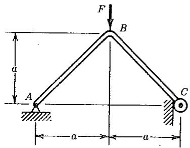
Problem 17.42 17.42 The angle frame shown has uniform bending stiffness EI. At C, a small frictionless roller contacts a vertical surface. (a) Solve for the vertical deflection at $C$ caused by force $F$ , using mechanics of materials methods. Assume that this deflection is small. (b) Solve by a computer program, for example, based on the algorithm described in Section 17.7. What difficulty appears in the first iterative cycle, and how will you overcome it? 17.43 The algorithm described in Section 17.7 can be applied to a plane body modeled by four-node quadrilaterals. Describe in detail how one might track the rigid-body motion of a quadrilateral and compute its d.o.f. $\{d'\}$ in a local coordinate system attached to the element. Assume that all displacements lie in the xy plane. 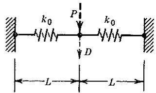17.44 When P and its displacement D are zero, the springs are unstressed (see sketch). Spring stiffness $k_{0}$ is constant. (a) Determine the secant stiffness (the ratio of $P$ to $D$ ) for small values of $D$ ( $D << L$ ). (b) What is the tangent stiffness for small values of $D$ ? (c) Determine an expression for the secant stiffness if $D$ may be moderate to large. (d) Describe an iterative way to calculate $D$ for a given $P$ , with particular emphasis on the first step. 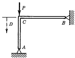17.45 The frame shown is built of slender members that may be assumed to remain linearly elastic at all times. Connections at $A$ and $B$ are frictionless pins. (a) Qualitatively sketch the anticipated relation between load $P$ and its vertical displacement $D$ . (b) How would you generate the $P$ versus $D$ relation numerically? That is, what difficulties do you anticipate, and how might you avoid or overcome them? 

text_image

k₀ P k₀ D L L

Problem 17.44 

text_image

P D C B A

Problem 17.45 # NUMERICAL ERRORS AND CONVERGENCE Sources of computational error are categorized. Methods of detecting and avoiding such errors are presented. The relation between element size and solution error is discussed. Tests of element quality are reviewed. # 18.1 INTRODUCTION. ERROR CLASSIFICATION Computed results are rarely exact. Some of the many reasons are as follows. We divide a structure into elements whose displacement fields exclude many of the physically possible deformation modes. The type, number, and shapes of elements may be chosen within a broad range of possibilities, and some choices are better than others. The computer represents numbers by a finite number of bits or digits. Numerical difficulties may arise even when the analyst makes no outright blunder in using a computer program. In this chapter we assume that there are no outright blunders, that is, that the program used is appropriate to the task at hand, that the program is free of bugs, that the choices of element types, shapes, and quadrature orders are suitable, and that elements pass patch tests and do not lock. Some choices remain, such as the specific type and number of elements, their arrangement, and the way in which relatively stiff regions are treated. How these choices are made can increase or decrease numerical error, which is caused by the inability of a computer to store and process numbers in infinite precision. There is no single definitive test of solution accuracy short of knowing the correct result by other means. A calculation that survives one error test may fail another. A usually reliable error test may fail in particular cases. For example, given a single-precision matrix [H], one may calculate $[X] = [H]^{-1}$ , then $[Y] = [X]^{-1}$ . If [Y] agrees with [H], one expects [X] to be correct. In fact, when [H] is a tenth-order Hilbert matrix $(H_{ij} = (i + j - 1)^{-1}$ , which is notoriously ill conditioned), one study found that [Y] = [H] to seven-digit accuracy, yet [X] had coefficients in error by three orders of magnitude [18.1]. Granted that some loss of precision is possible or even likely in finite element calculations, one should not introduce gratuitous errors: numerical constants, such as $\pi$ and Gauss point coordinates and weights, should be written with as many accurate digits as the machine can accommodate. Terminology. The following terms are useful in subsequent discussion [18.2]. This abbreviated list shows at once that there are several aspects to the study of numerical errors. Modeling error refers to the difference between a physical system and its math- ematical model. For example, an actual plate may be mathematically modeled by Kirchhoff plate theory. Numerical analysis is performed on the mathematical model. It is this analysis that is subject to the following errors. Discretization error refers to the error caused by representing the infinitely many d.o.f. of a continuous mathematical model by a finite number of d.o.f. in its discretized form. For example, the aforementioned Kirchhoff plate is divided into finite elements, thus introducing discretization error. Round-off error is caused by use of a finite number of bits or digits to represent real numbers. The last digit retained may be rounded or may be obtained by simple truncation (chopping). The round-off limit is the smallest floating point number $\epsilon$ such that, in the computer, $1.0 + \epsilon > 1.0$ . For example, one may find $\epsilon = 7(10^{-15})$ on some machine in double-precision arithmetic. Inherited error at any stage of calculation is the sum of previous discretization and round-off errors. Manipulation error refers to round-off error introduced by an algorithm. For example, an equation solver performs numerical operations such as $A_{22} - (A_{21}/A_{11})A_{12}$ , where the $A_{ij}$ are matrix coefficients. The division and multiplication are each followed by rounding of the result to computer-word length, and the subtraction may lose several significant digits if $A_{22}$ and $(A_{21}/A_{11})A_{12}$ are almost equal. For example, if $R = D_{1} - D_{2}$ , where $D_{1} = 1.23456$ and $D_{2} = 1.23455$ , then $R = 1.00000(10^{-5})$ , which contains but one significant digit in its six-digit mantissa and is therefore far less accurate than either $D_{1}$ or $D_{2}$ . In a finite element context, inherited error is present after disparate element stiffnesses are added to form structural stiffness coefficients, and manipulation error is produced by solving the equations. Alternative terms for these errors are truncation and rounding. Inherited error and manipulation error have the same source: the round-off limit is not zero. # 18.2 ILL-CONDITIONING Concepts from Algebra. Consider the set of equations $$ \left[ \begin{array}{c c} 1. 0 0 & - 1. 0 0 \\ - 1. 0 0 & 1. 0 2 \end{array} \right] \left\{ \begin{array}{l} x \\ y \end{array} \right\} = \left\{ \begin{array}{c} 4. 0 0 \\ - 2. 0 0 \end{array} \right\} \quad \text { for which } \quad \left\{ \begin{array}{l} x \\ y \end{array} \right\} = \left\{ \begin{array}{l} 1 0 4 \\ 1 0 0 \end{array} \right\} \tag {18.2-1} $$ and the very similar set of equations $$ \left[ \begin{array}{c c} 1. 0 0 & - 1. 0 0 \\ - 1. 0 0 & 1. 0 1 \end{array} \right] \left\{ \begin{array}{l} x \\ y \end{array} \right\} = \left\{ \begin{array}{c} 4. 0 0 \\ - 2. 0 0 \end{array} \right\} \quad \text { for which } \quad \left\{ \begin{array}{l} x \\ y \end{array} \right\} = \left\{ \begin{array}{l} 2 0 4 \\ 2 0 0 \end{array} \right\} \tag {18.2-2} $$ A 1% change in one coefficient has changed the results by a factor of two. These equation sets are both ill conditioned, which means that their solutions are sensitive to small changes in either the coefficient matrix or the vector of constants. The solution of Eq. 18.2-1 can be regarded as the intersection point in xy space of two straight lines, one representing the equation x - y = 4 and the other representing the equation $-x + 1.02y = -2$ . When plotted, the two lines are seen to be almost parallel. Accordingly, when the second equation is changed to $-x + 1.01y = -2$ (Eq. 18.2-2), the second line is rotated slightly, and the intersection point changes markedly. In matrix terminology, the rows of an ill-conditioned matrix are almost linearly dependent. For 2 by 2 systems such as Eqs. 18.2-1 and 18.2-2, this means that the second row of the coefficient matrix is almost a scalar multiple of the first row. A Gauss elimination solution of these equations changes the second diagonal coefficient in Eq. 18.2-1 to 1.02 - 1.00 = 0.02. If only two digits were retained, all coefficients would be represented as 1.0 and the matrix would be singular. Gauss elimination would produce 1.0 - 1.0 = 0.0 as the second diagonal coefficient and the computation y = 2.0/0.0 would be attempted. 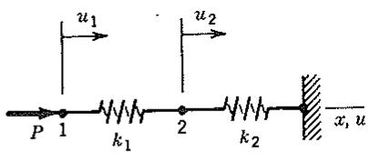Comparatively Flexible Support. In Fig. 18.2-1, the circumstance $k_{1} >> k_{2}$ promotes ill-conditioning but the circumstance $k_{2} >> k_{1}$ does not. This is easy to see by examining the structure equations [K] $\{D\} = \{R\}$ , which are $$ \left[ \begin{array}{c c} k _ {1} & - k _ {1} \\ - k _ {1} & k _ {1} + k _ {2} \end{array} \right] \left\{ \begin{array}{l} u _ {1} \\ u _ {2} \end{array} \right\} = \left\{ \begin{array}{l} P \\ 0 \end{array} \right\} \tag {18.2-3} $$ The rows of [K] are almost linearly dependent if $k_{1} >> k_{2}$ , but not if $k_{2} >> k_{1}$ . In a Gauss elimination solution, we calculate the reduced coefficient $K_{22} = (k_{1} + k_{2}) - k_{1}$ , which yields an inaccurate result if $k_{1} >> k_{2}$ and $k_{2} / k_{1}$ is close to the round-off limit. To make the point numerically, imagine that $k_{1} = 40$ and $k_{2} = 0.0014$ . If the last digit of $k_{2}$ is to appear in the number $k_{1} + k_{2}$ , the computer word mantissa must store at least six digits and $k_{1}$ must be represented as 40.0000. (That $k_{1}$ is not physically known to six-digit accuracy does not matter.) If five digits were stored, Gauss elimination would produce a reduced $K_{22}$ of 0.0010 rather than the correct reduced value $K_{22} = 0.0014$ . If only four digits were stored, $k_{1} + k_{2}$ would be represented as 40.00, and [K] would be singular. That is, [K] would represent only the single spring $k_{1}$ , unsupported and free to translate as a rigid body. In the foregoing example, the modeling and discretization errors are zero, but round-off produces an inherited error in [K] that becomes obvious during subsequent manipulations. In summary, and in structural terminology, a major cause of ill-conditioning in practical finite element models is a large difference in stiffnesses, with the stiffer region being supported by the more flexible region. This circumstance shifts essential numerical information to the latter digits of stiffness coefficients $K_{ij}$ . These latter digits may be so few in number that the solution is worthless. Physically, 

text_image

u₁ u₂ P 1 k₁ 2 k₂ x, u

Figure 18.2-1. Two-d.o.f. structure with linear springs of stiffness $k_{1}$ and $k_{2}$ . 

text_image

v₁ θ₁ u₁ 1 2 v₂ θ₂ u₂

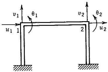
Figure 18.2-2. A plane frame with six nonzero d.o.f. the stiffer region has one or more displacement states that are almost rigid-body motions within a more flexible supporting structure. The limiting case is a structure without any supports: it has only rigid-body motion in static analysis, and its stiffness matrix is singular. In nonstructural problems, similar difficulties may arise. For example, in heat conduction analysis one might encounter a region of high conductivity imbedded in a region of low conductivity. One way to avoid difficulty is to use longer computer words—that is, double precision rather than single precision. But if equations are generated by use of single-precision arithmetic and are ill conditioned, will it help to solve them by use of double-precision arithmetic? From our discussion, the answer is no. Information already discarded cannot be recovered by subsequent manipulation, however accurately done. Structures susceptible to ill-conditioning include thin shells, for which membrane stiffness is much greater than bending stiffness. For the same reason, the frame of Fig. 18.2-2 may be troublesome: the axial stiffness of horizontal member 1–2 greatly exceeds its bending stiffness, so horizontal load will produce $u_{1} \approx u_{2}$ . For such a problem it is usually best to enforce $u_{1} = u_{2}$ by application of a constraint. Thus, a source of ill-conditioning is removed. 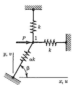An Important Special Case. The three-member structure in Fig. 18.2-3a has springs of stiffness $\alpha k$ and k. If $\alpha$ is large, a stiff structure (the spring of stiffness $\alpha k$ ) is supported against rigid-body motion by a flexible structure (the springs of stiffness k). Structural equations of this system are $$ \left[ \begin{array}{c c} k (1 + \alpha c ^ {2}) & k \alpha c s \\ k \alpha c s & k (1 + \alpha s ^ {2}) \end{array} \right] \left\{ \begin{array}{l} u _ {1} \\ v _ {1} \end{array} \right\} = \left\{ \begin{array}{l} P \\ 0 \end{array} \right\} \quad \text { where } \quad \begin{array}{l} c = \cos \beta \\ s = \sin \beta \end{array} \tag {18.2-4} $$ In $u_{1}v_{1}$ space, the straight lines corresponding to these two equations have the respective slopes $$ - \frac {1 + \alpha c ^ {2}}{\alpha c s} \quad \text { and } \quad - \frac {\alpha c s}{1 + \alpha s ^ {2}} \tag {18.2-5} $$ If $\alpha >> 1$ , the two slopes are nearly the same, and ill-conditioning is therefore 

text_image

k P 1 k αk β y, v x, u

(a) 

text_image

y, v D E n A B x, u C t

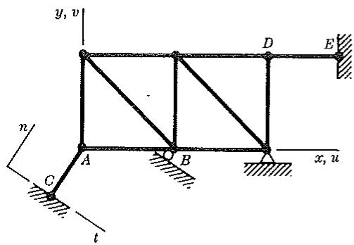
(b) Figure 18.2-3. (a) Three-spring structure, having d.o.f. $u_{1}$ and $v_{1}$ at node 1. (b) Skew supports at A and B in a plane truss. indicated. However, there are two exceptions: for $c = 0$ ( $\beta = \pi/2$ ) and for $s = 0$ ( $\beta = 0$ ), spring $\alpha k$ contributes no off-diagonal terms to the structure stiffness matrix, and the equations are well conditioned for any value of $\alpha$ . The practical implication of the foregoing analysis is as follows. In Fig. 18.2-3b, let each node i have the usual d.o.f. $u_{i}$ and $v_{i}$ . A very stiff bar DE approximates the constraint $u_{D} = 0$ but does not produce ill-conditioning because $\beta = 0$ for bar DE. At node A, imagine that the constraint of zero n-direction motion is desired. One can approximate this constraint condition by inserting a very stiff bar AC. This invites ill-conditioning if d.o.f. at A are x- and y-direction displacements, but not if d.o.f. at A are n- and t-direction displacements (introduced by coordinate transformation prior to assembly of elements). However, if coordinate transformation has been invoked, one may as well simply set the n-direction displacement at A to zero (as is implied at node B). Avoiding Trouble. We have seen that large stiffness differences may be troublesome. The ideal, not always attainable in practice, is a model without large discrepancies in stiffness. Arbitrary adjustments in modeling may be appropriate. A comparatively stiff region may be modeled as perfectly rigid by use of a constraint transformation, as has been noted in connection with Fig. 18.2-2. On the other hand, perhaps a stiff region can be made more flexible. For example, in Fig. 18.2-2 one may be able to decrease the axial stiffness $AE / L$ of bar 1-2 by a factor of (say) 100: if the members are slender, bending will still dominate the solution, and $u_{1}$ and $u_{2}$ will still greatly exceed the relative motion $u_{2} - u_{1}$ . Another possibility in modeling is to use relative motions, rather than absolute motions, for troublesome d.o.f. For example, in Fig. 18.2-1 one could introduce the d.o.f. $u_{r} = u_{1} - u_{2}$ . Instead of Eqs. 18.2-3 we now have $$ \left[ \begin{array}{l l} k _ {1} & 0 \\ 0 & k _ {2} \end{array} \right] \left\{ \begin{array}{l} u _ {r} \\ u _ {2} \end{array} \right\} = \left\{ \begin{array}{l} P \\ P \end{array} \right\} \tag {18.2-6} $$ Equations 18.2-6 are well conditioned for all values of $k_{1}$ and $k_{2}$ . Equations 18.2-6 must be obtained by using $u_{r}$ as a d.o.f. in element formulation and assembly. No purpose would be served by introducing $u_{r}$ by coordinate transformation of the assembled equations, Eqs. 18.2-3, as the coefficient $k_{1} + k_{2}$ already contains the error we seek to avoid. After a good finite element model is prepared, subsequent manipulation errors may be negligible. However, it is recommended that double-precision arithmetic be used for all phases of a finite element analysis, unless the round-off limit is about $10^{-14}$ in single precision or the problem has very few d.o.f. # 18.3 THE CONDITION NUMBER A numerical measure of the ill-conditioning in a coefficient matrix $[K]$ is the condition number, denoted here by $C(\mathbf{K})$ . A large condition number warns that a finite element solution may contain appreciable error: the anticipated error may be realized for some systems and some loadings but not for others. Definition and Interpretation. The spectral condition number of a matrix $[K]$ , which we will call simply the condition number, is defined as $$ C (\mathbf {K}) = \frac {\lambda_ {\max}}{\lambda_ {\min}} \tag {18.3-1} $$ where $\lambda_{\max}$ and $\lambda_{\min}$ are largest and smallest eigenvalues of [K]. (It is best to scale [K] before calculating $C(\mathbf{K})$ , as described in connection with Eqs. 18.3-3 to 18.3-6.) It can be shown [18.1] that for each power of ten in the ratio $\lambda_{max}/\lambda_{min}$ , the operations of equation solving lose about one digit of accuracy in the displacement mode associated with $\lambda_{min}$ . In a direct method of solving equations, such as Gauss elimination, the difficulty may materialize near the end of the forward-reduction phase, when the difference is computed between two numbers that are almost equal. Error contamination spreads during the back-substitution phase. The estimated accuracy loss is $$ \text { accurate digits lost } \approx \log_ {1 0} \frac {\lambda_ {\max}}{\lambda_ {\min}} = \log_ {1 0} C (\mathbf {K}) \tag {18.3-2} $$ For example, imagine that $C(\mathbf{K}) = 10^{5}$ . If computer words have seven-digit capacity, only two reliable digits may remain in the computed displacements. With fourteen-digit capacity, nine accurate digits may remain. The estimate given by Eq. 18.3-2 is based on the inherited error, caused by round-off, that exists at the outset of equation solving. The estimate does not include the manipulation error of the solution algorithm. 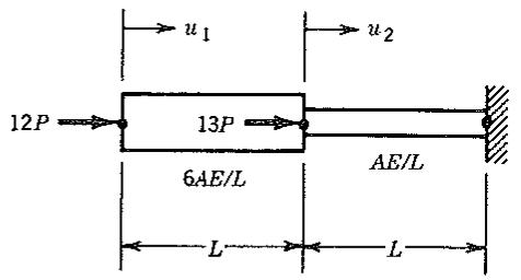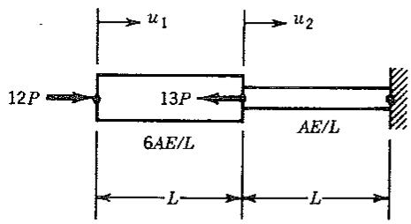For stress analysis purposes, the estimate in Eq. 18.3-2 may be pessimistic because it ignores the load vector. Consider Fig. 18.3-1. For both load cases shown, the percentage errors in computed values of $u_{1}$ and $u_{2}$ are larger than the percentage error in the computed relative displacement $u_{1} - u_{2}$ . In stress analysis one seeks the largest strains. The strain of largest magnitude is $u_{2}/L$ in Fig. 18.3-1a but is $(u_{1} - u_{2})/L$ in Fig. 18.3-1b. Accordingly, ill-conditioning may be of little consequence in Fig. 18.3-1b. In general, for stress analysis one should estimate the number accurate digits lost as $\log_{10}(\lambda_{\max}/\lambda_{k})$ , where $\lambda_{k}$ is the lowest eigenvalue of [K] whose associated eigenmode is not approximately orthogonal to the load vector. Usually $\lambda_{k} = \lambda_{min}$ , but not necessarily. Thus, in Fig. 18.3-1b, the loss of digits in the strain $(u_{1} - u_{2})/L$ is more accurately predicted by using 

text_image

u₁ → u₂ 12P → 13P → AE/L 6AE/L L → L

(a) 

text_image

u₁ → u₂ 12P → 13P ← AE/L 6AE/L L ← L

(b) Figure 18.3-1. Two different load sets on a two-d.o.f. bar structure. The respective elements have axial stiffnesses 6AE/L and AE/L. the $\lambda_{k}$ associated with the eigenmode in which $u_{1}$ and $u_{2}$ are of opposite sign than by using $\lambda_{k} = \lambda_{\min}$ (in whose eigenmode $u_{1}$ and $u_{2}$ are of the same sign). Calculation and Scaling. Besides ignoring the load vector, Eq. 18.3-2 may overestimate error because $C(\mathbf{K})$ is “artificially” high. In Fig. 18.2-1 for example, $C(\mathbf{K})$ is large when $k_{1} >> k_{2}$ and when $k_{2} >> k_{1}$ , yet the case $k_{2} >> k_{1}$ is well conditioned. One can arrange for $C(\mathbf{K})$ to be large only when [K] is truly ill conditioned by scaling [K] before calculating $C(\mathbf{K})$ , as follows. One constructs a diagonal scaling matrix [S] from diagonal coefficients in [K], then transforms [K] to the scaled matrix $[K_{s}]$ : $$ [ \mathrm{K} _ {s} ] = [ \mathrm{S} ] [ \mathrm{K} ] [ \mathrm{S} ] \quad \text { where } \quad S _ {i i} = \frac {1}{\sqrt {K _ {i i}}} \tag {18.3-3} $$ Diagonal coefficients of $[\mathbf{K}_s]$ are unity. The extreme eigenvalues $\lambda_{\max}$ and $\lambda_{\min}$ of $[\mathbf{K}_s]$ are to be used in Eq. 18.3-2. The eigenvalue problem that yields $\lambda_{\mathrm{max}}$ and $\lambda_{\mathrm{min}}$ of the scaled matrix $[\mathbf{K}_s]$ is $$ \left(\left[ \mathbf {K} _ {s} \right] - \lambda \lceil \mathbf {I} \rceil\right) \{\mathbf {D} \} = \{\mathbf {0} \} \tag {18.3-4} $$ which may be regarded as a vibration problem with a unit mass matrix and natural frequencies $\omega_{i}^{2} = \lambda_{i}$ . An alternative form, which yields the same eigenvalues as Eq. 18.3-4, is produced by substituting $\{D\} = \left[S\right]^{-1}\{D_{1}\}$ and premultiplying by $[S]^{-1}$ . Thus [18.3] $$ \left(\left[ \mathrm{S} \right] ^ {- 1} \left[ \mathrm{K} _ {s} \right] \left[ \mathrm{S} \right] ^ {- 1} - \lambda \left[ \mathrm{S} \right] ^ {- 1} \left[ \mathrm{S} \right] ^ {- 1}\right) \left\{\mathrm{D} _ {1} \right\} = \{0 \} \tag {18.3-5} $$ which is the same as $$ ([ \mathbf {K} ] - \lambda [ K _ {1 1} K _ {2 2} \dots K _ {n n} ]) \{\mathbf {D} _ {1} \} = \{\mathbf {0} \} \tag {18.3-6} $$ Therefore, $\lambda_{max}$ and $\lambda_{min}$ of the scaled matrix $[K_{s}]$ can be calculated using the unscaled [K] and a diagonal “mass” matrix that is simply the principal diagonal of [K]. Equation 18.3-6 shows why an isolated stiff region raises $C(\mathbf{K})$ : an isolated large “mass” $K_{ii}$ , if not held by supports, reduces the lowest “frequency” but has little effect on the highest “frequency.” Scaling is used only to avoid obtaining an unrealistically pessimistic result from Eq. 18.3-2 because of “artificial” ill-conditioning. Scaling need not be applied to the [K] used in solving equations. Scaling of [K] has no effect on the accuracy of a direct-solution algorithm such as Gauss elimination, assuming that the scaling process itself introduces no manipulation error, and provided that the choice of pivots and the sequence of eliminations are unchanged [18.4]. Because Eq. 18.3-2 is only an approximation, $\lambda_{max}$ and $\lambda_{min}$ need not be computed accurately. A close upper bound on $\lambda_{max}$ of $[K_{s}]$ can be obtained from the Gerschgorin bound, Eq. 13.10-17. Thus we add the magnitudes of coefficients in each row of $[K_{s}]$ , then choose the largest such row sum, that is, $$ \lambda_ {\max} \approx \max Q _ {i} \quad \text { where } \quad Q _ {i} = \sum_ {j = 1} ^ {n} \left| K _ {s i j} \right| \tag {18.3-7} $$ where n is the order of $[K_{s}]$ . Unfortunately, there is no corresponding simple estimate of $\lambda_{min}$ . The expense of computing $\lambda_{min}$ is comparable to the expense of solving equations, which means that Eq. 18.3-2 does not provide an inexpensive a priori estimate of solution accuracy. Causes of Ill-Conditioning. A finite element model tends to produce ill-conditioned equations if an element or a patch of elements can respond to loads with large rigid-body motion but little deformation. Examples include (a) high-modulus inclusions, (b) plate elements that allow transverse shear strain but have large transverse shear stiffness because they are thin, (c) elements of severe shape distortion or large aspect ratio, and (d) stiff supports such as spring $\alpha k$ in Fig. 18.2-3. (Analogous difficulties can appear in nonstructural problems.) In the foregoing cases one can reduce or eliminate the trouble by changing the model. In the respective examples, one can (a) make the inclusion rigid by applying constraints, (b) use thin-plate elements or arbitrarily decrease the shear stiffness, (c) remodel using more regular and compact element shapes, and (d) use differently directly d.o.f. at the offending node. Ill-conditioning of a stiffness matrix may also be caused by mixing elements of different size and by using a fine mesh. It has been found that [18.5] $$ C (\mathbf {K}) = b \left(\frac {h _ {\max}}{h _ {\min}}\right) ^ {2 m - 1} N ^ {2 m / n} \tag {18.3-8} $$ where $b =$ a positive constant independent of $h_{\max}$ and $h_{\min}$ , $$ h _ {\min} = \text { smallest node spacing in any element of the mesh }, $$ $$ h _ {\max} = \text { greatest node spacing in any element of the mesh }, $$ $$ N = \text { number of elements }, $$ $$ 2 m = \text { differential equation order }, $$ $$ n = \text { dimensionality }. $$ To elaborate, the differential equation that describes the physical problem uses dispalements as dependent variables, has 2m as the highest derivative of the dependent variable(s), and requires n independent variables. As examples, for an axially loaded bar, 2m/n = 2/1; for a beam, 2m/n = 4/1; in plane stress, 2m/n = 2/2; in thin-plate bending, 2m/n = 4/2; in three-dimensional solids, 2m/n = 2/3; for a thin shell, 2m/n = 4/3. Thus, in a beam problem, if the length ratio $h_{max}/h_{min}$ of elements is changed from 1/1 to 10/1, $C(\mathbf{K})$ increases by a factor of 1000. If the number of elements is doubled, $C(\mathbf{K})$ increases by a factor of 16. If both of these changes are made, $C(\mathbf{K})$ increases by a factor of 16,000. As a practical matter, we would like to know the dependencies of the condition number on important mesh and problem parameters. For the unscaled stiffness matrix, Fried [18.5] has shown that $$ \left(\frac {1}{\lambda_ {1} c _ {\max}}\right) \frac {\max _ {l \leq \ell \leq N} \left(\Lambda_ {\ell} ^ {k}\right)}{\max _ {l \leq \ell \leq N} \left(\Lambda_ {\ell} ^ {n}\right)} \leq C (\mathbf {K}) \leq \left(\frac {c _ {\max}}{\lambda_ {1}}\right) \frac {\max _ {l \leq \ell \leq N} \left(\Lambda_ {\ell} ^ {k}\right)}{\min _ {l \leq \ell \leq N} \left(\lambda_ {\ell} ^ {n}\right)} \tag {18.3-9} $$ where, using unscaled element stiffness and mass matrices, $$ \begin{array}{l} \Lambda_ {\ell} ^ {k}, \Lambda_ {\ell} ^ {m} = \text { maximum eigenvalue of the stiffness and mass matrices }, \\ \text { respectively, of element } \ell , \end{array} $$ $$ \lambda_ {\ell} ^ {m} = \text { minimum eigenvalue of the mass matrix of element } \ell , $$ $$ \lambda_ {1} = \text { minimum eigenvalue of the continuous problem }, $$ $$ N = \text { number of elements in the structure }, $$ $$ c _ {\max} = \text { maximum number of elements meeting at a single node. } $$ The mass matrix cited need not be the consistent mass matrix; it may be lumped provided that no $\lambda_{\ell}^{m}$ is zero because a d.o.f. is assigned zero mass. Alternative notation for $\lambda_{1}$ is $\omega_{1}^{2}$ , where $\omega_{1}$ is the fundamental vibration frequency of the actual structure. Mass density cancels in the denominators and so may be taken as unity. One can use estimates of $\Lambda_{\ell}^{k}$ and $\Lambda_{\ell}^{m}$ obtained from the Gershgorin bound, Eq. 13.10-17. Hence, if $\lambda_{1}$ is known, Eq. 18.3-9 provides estimated numerical bounds on $C(\mathbf{K})$ . We see from Eq. 18.3-9 that the bound on $C(\mathbf{K})$ becomes less certain as more elements are connected to a node. However, $c_{max}$ is typically 4, 6, or even 8, which indicates a probable uncertainty of about one digit in $\log_{10} C(\mathbf{K})$ . The condition number may be strongly affected by Poisson's ratio $\nu$ . Fried [18.18] has shown that $b$ in Eq. 18.3-8 is given by $$ b = \frac {b _ {1}}{1 - 2 \nu} \tag {18.3-10} $$ where $b_{1}$ is a constant that is independent of E and $\nu$ (provided that E and $\nu$ are constant throughout the mesh). Equation 9.4-12 shows that b is a penalty number $\alpha$ , that is, $\alpha = b/3b_{1}$ . Near the incompressibility limit of $\nu = 0.5$ , Eq. 18.3-10 can increase $C(\mathbf{K})$ by orders of magnitude. If computer words carry about p digits each, and if the value of $\alpha$ or b approaches $10^{p/2}$ as suggested at the end of Section 9.4, then we might expect an accuracy loss of almost p/2 digits in the solution process. Such a loss may be of concern if pressures in nearly incompressible media are computed by the penalty method (see Eqs. 9.5-1 and 9.6-2), for the following reason. Strain $\epsilon_{V}$ in Eq. 9.5-1 is small because strains $u_{,x}$ , $v_{,y}$ , and $w_{,z}$ almost cancel one another when added to produce $\epsilon_{V}$ , even when using computer words of p-digit accuracy. We now propose to calculate $\epsilon_{V}$ by adding three strains that are each accurate in only about the leading p/2 digits. If $\epsilon_{V}$ is to be computed with useful accuracy, a more rigorous analysis suggests that $\alpha$ should be approximately $10^{p/3}$ . In practice the estimate $\alpha \approx 10^{p/3}$ appears to be sufficiently pessimistic that a value of $\alpha$ approaching $10^{p/2}$ can usually be used. # 18.4 DIAGONAL DECAY ERROR TESTS Here we describe a simple and inexpensive test for round-off errors that appear during a direct method of solving equations, such as the Gauss elimination method. The test can warn of possible trouble and can be used to terminate execution if serious trouble is indicated [18.6]. Assume that the coefficient matrix [K] is symmetric and positive definite. Then, as each equation is processed, that is, as each unknown is eliminated, a subtraction operation reduces the magnitude of diagonal coefficients $K_{ii}$ that correspond to d.o.f. i yet to be eliminated (however, each $K_{ii}$ remains positive). Thus, each $K_{ii}$