text_image

L = 2.40 P = 100 0.10 E = 10^4 w 0.40 v = 0.25

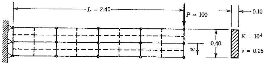
Figure 18.7-4. End-loaded cantilever beam. Mesh N = 8 is shown. Mesh N = 32 is suggested by dashed lines. All elements are bilinear. necessary for exactness do not prevail. Rather than regarding $\phi^0$ as the exact value, it seems preferable to regard $$ e = \frac {\phi_ {2} - \phi^ {0}}{\phi^ {0}} 100\% \tag{18.7 - 5} $$ as an estimate of percentage errors in mesh $h_{2}$ . Example: Regular Refinement. The cantilever beam problem shown in Fig. 18.7-4 was solved using three different meshes and three different formulations for each mesh. Results are presented in Fig. 18.7-5 and in Table 18.7-1 using the following notation. Element stiffness matrices were integrated using 2 by 2 quadrature (“Full”) or one-point quadrature (“Reduced” and “H-G”), where “H-G” refers to hourglass control (see Eq. 6.12-4). No mechanism is possible in the reduced-integration case because of complete fixity at the left end. The problem was solved on a microcomputer whose capacity did not permit the use of a finer mesh than N = 128. 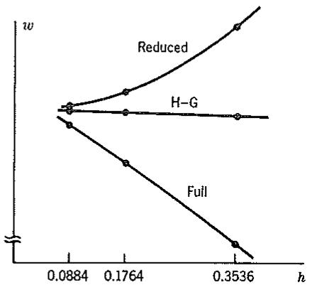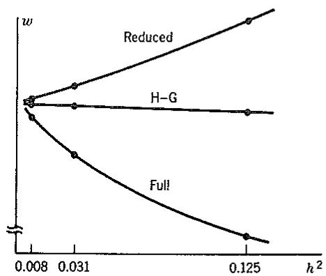Figure 18.7-5 suggests that $e = O(h)$ for the full-integration case and $e = O(h^{2})$ for the reduced-integration case. Nevertheless, all extrapolated values in Table 18.7-1 were computed using p = 2 in Eq. 18.7-4. 

line

| h | w (Reduced) | w (H-G) | w (Full) | | ------- | ----------- | ------- | -------- | | 0.0884 | ~0.8 | ~0.8 | ~0.8 | | 0.1764 | ~1.0 | ~0.8 | ~0.6 | | 0.3536 | ~1.5 | ~0.8 | ~0.4 |

(a) 

line

| h² | w (Reduced) | w (H−G) | w (Full) | | ------ | ----------- | ------- | -------- | | 0.008 | 0 | 0 | 0 | | 0.031 | ~0.5 | ~0.5 | ~0.5 | | 0.125 | ~1.0 | ~0.5 | ~0.5 |

(b) Figure 18.7-5. Plots of data from Table 18.7-1, for the problem of Fig. 18.7-4: (a) w versus h, (b) w versus $h^{2}$ . TABLE 18.7-1. COMPUTED DEFLECTION W IN FIG. 18.7-4. BEAM THEORY, INCLUDING TRANSVERSE SHEAR DEFORMATION, GIVES $w = (PL^{3}/3EI) + (6PL/5AG) = 8.640 + 0.180 = 8.820$ . EXTRAPOLATION IS BASED ON p = 2 IN EQ. 18.7-4.

Mesh Data		Computed Results (w)			Extrapolated Results (w)
N	$h = 1/N^{1/2}$	Full	Reduced	H-G	Full	Reduced	H-G
8	0.3536	4.562	11.440	8.572	7.978	8.617	8.768
32	0.1768	7.124	9.323	8.719	8.695	8.788	8.788
128	0.0884	8.302	8.922	8.771

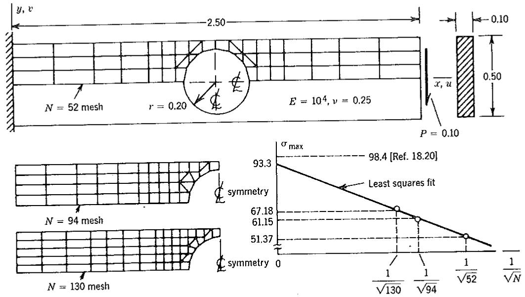
Example: Irregular Refinement. The beam in Fig. 18.7-6 contains a large central hole. We seek the largest principal stress. Each mesh shown is composed of bilinear elements, for which a 2 by 2 integration rule was used. Load $P$ is uniformly distributed across the right end. The upper half of the beam was modeled, with all nodes on $x = 0$ fixed and all nodes on $y = 0$ allowed only vertical displacement. Even so, the microcomputer could not accommodate regular mesh refinement. The meshes shown violate most rules of regular refinement. Indeed, the meshes could be substantially improved because they are undesirably coarse close to the hole and unnecessarily fine far from the hole. Stresses were evaluated at element centers. What is plotted as $\sigma_{\max}$ is the largest element center stress from each mesh, regardless of the element in which it appears. For pure bending load, photoelastic data indicate that $\sigma_{max}$ appears at the top edge of the hole and is $\sigma_{max} = 98.4$ [18.20]. One can perhaps assume that the error in $\sigma_{max}$ is $O(h)$ . Hence, a least squares fit of a straight line to the three data points yields 

other

| Dimension | Value | | ----------------- | ------ | | Width (N) | 52 mesh | | Radius (r) | 0.20 | | Total Width (N) | 94 mesh | | Thickness (N) | 130 mesh | | Stress (σ_max) | 93.3 | | Least Squares Fit | 67.18 | | Constant (σ_max) | 61.15 | | Constant (σ_max) | 51.37 | | Constant (σ_max) | 1 | | Constant (σ_max) | 1/√130 | | Constant (σ_max) | 1/√94 | | Constant (σ_max) | 1/√52 | | Constant (σ_max) | 1/√N |

Figure 18.7-6. Cantilever beam with a large central hole. Each mesh is symmetric about both centerlines. Results of irregular mesh refinement are shown. (The authors are grateful to S-C. Liang and D. Rusche for doing the computations.) 

natural_image

Geometric diagram of two adjacent rectangles with diagonal lines (no text or symbols)

Original mesh 

natural_image

Pure geometric grid pattern with diagonal lines and dots, no text or symbols present

h refinement 

natural_image

Pure geometric diagram of a rectangle divided into two sections by diagonal lines (no text or symbols)

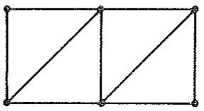
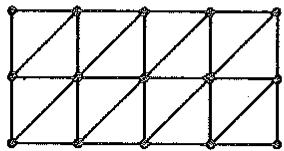
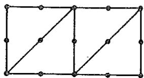
p refinement Figure 18.7-7. The $h$ and $p$ versions of refinement of a plane mesh. $\sigma_{max} = 93.3$ , as shown. This extrapolated result is remarkably good, and perhaps somewhat fortuitous. At the very least, the plotted results show that none of the three meshes by itself yields a reliable result. The h version and the p version. The h and p versions of the finite element method are different ways of adding d.o.f. to the model, so as to reduce discretization error in a subsequent analysis. The h version refers to decreasing the characteristic length (h) of elements, by dividing each existing element into two or more elements, but without changing the types of elements used. The p version refers to increasing the degree of the highest complete polynomial (p) in elements, by adding nodes to elements, adding d.o.f. (e.g., derivative d.o.f.) to nodes, or both, but without changing the number of elements used. In Fig. 18.7-7, the next stage of p refinement might be to add derivative d.o.f. without changing the number of nodes. A sequence of successively refined meshes produces convergence toward correct results. The process is known as h convergence or p convergence, depending on the method of adding d.o.f. A computer program is termed “adaptive” if addition of d.o.f. and reanalysis can be accomplished with a minimum of direction from the analyst. The program is called “self-adaptive” if it can automatically decide where additional d.o.f. are most needed in the model, prepare a suitable new model, reanalyze, and keep repeating the process until a preselected convergence tolerance is achieved $[18.12,18.13]$ . Adaptive h refinement can continue until limits imposed by computer capacity and numerical noise are reached. Adaptive p refinement can continue until the highest-order polynomial coded in the program is used. Error estimates and monotonic convergence of successive solutions are made possible by completely regular mesh refinement, which is known in the present context as a “hierarchical” procedure. Hierarchical refinement produces a mesh that allows, as special cases, all displacement modes that were possible in the unrefined mesh. Both refinements in Fig. 18.7-7 are hierarchical. With either the h version or the p version, clever programming can incorporate computations done in the preceding mesh rather than repeating them entire for the current mesh. # 18.8 TESTS OF ELEMENT QUALITY Eigenvalue Test. The eigenvalue test is one of several tests of element quality. The test can detect zero-energy deformation modes, lack of invariance, and absence of rigid-body motion capability. It can also be used to estimate the relative quality of competing elements $[18.14,18.15]$ . We will describe the calculations first and then comment on how to interpret results. Let loads $\{\bar{r}\}$ applied to element nodes be proportional to element nodal displacements $\{d\}$ through a factor $\lambda$ : $$ [ \mathbf {k} ] \{\mathbf {d} \} = \{\overline {{{\mathbf {r}}}} \} = \lambda \{\mathbf {d} \} \quad \text { or } \quad ([ \mathbf {k} ] - \lambda [ \mathbf {I} ]) \{\mathbf {d} \} = \{\mathbf {0} \} \tag {18.8-1} $$ This is an eigenproblem. Eigenvalues $\lambda_{i}$ are called eigenvalues of [k]. There are as many $\lambda_{i}$ as there are d.o.f. in $\{\mathbf{d}\}$ . Not all $\lambda_{i}$ need be different. To each $\lambda_{i}$ there corresponds an eigenvector $\{\mathbf{d}\}_{i}$ . If each $\{\mathbf{d}\}_{i}$ is normalized so that $\{\mathbf{d}\}_{i}^{T}\{\mathbf{d}\}_{i}=1$ , premultiplication of Eq. 18.8-1 by $\{\mathbf{d}\}_{i}^{T}$ yields $$ \{\mathbf {d} \} _ {i} ^ {T} [ \mathbf {k} ] \{\mathbf {d} \} _ {i} = \lambda_ {i} \quad \text { or } \quad 2 U _ {i} = \lambda_ {i} \tag {18.8-2} $$ where $U_{i}$ is strain energy in the element when its nodal d.o.f. are the normalized displacements $\{d\}_{i}$ (see Eq. 3.3-9). Usually the element is unrestrained for the eigenvalue test so that [k] is the complete element stiffness matrix. In an existing computer program, one can conveniently compute the $\lambda_{i}$ as the squared natural vibration frequencies of an unsupported element that has unit mass attached to each d.o.f. in $\{d\}$ . Note that $\lambda_{i}$ is unchanged if the deformation is reversed—that is, if $\{d\}_{i}$ is replaced by $-\{d\}_{i}$ . Equation 18.8-2 shows that [k] should yield $\lambda_{i}=0$ when $\{d\}_{i}$ represents any rigid-body motion. There are three linearly independent rigid-body motions possible in the plane. Therefore three of the $\lambda_{i}$ should be zero for a plane element. Six should be zero for a general solid or shell element, but only one for a solid or shell of revolution element (if only axially symmetric states are permitted). Zero-energy modes (mechanisms) also yield zero eigenvalues. The associated $\{d\}_{i}$ may appear in combination with the $\{d\}_{i}$ of a rigid-body motion. In testing an element, we first check that [k] has as many $\lambda_{i}=0$ values as expected. Too few suggests that the element lacks a desired capability for rigid-body motion without strain. Too many suggests the presence of one or more mechanisms. Nonzero eigenvalues are real and positive if $[k]$ is symmetric and positive semidefinite. If eigenvalues change when the element is reoriented in global coordinates, the element is not geometrically isotropic. Similar modes, such as the flexural modes of Fig. 18.8-1, should be associated with equal eigenvalues if the material is isotropic. 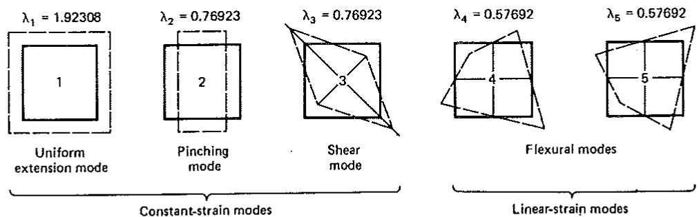Eigenvalues of $[k]$ can sometimes be used to compare different formulations of a given element type, for example, isoparametric versus hybrid formulations of  Figure 18.8-1. Nonzero eigenvalues and corresponding eigenvectors (deformation modes) of a square bilinear element in plane strain [18.16]. $E = 1.0$ , $\nu = 0.3$ , side length $= 1.0$ . a four-node plane element. Properly formulated elements of the same size, shape, and material properties should be equally stiff in their constant strain modes. Their stiffness matrices should therefore have eigenvalues in common. Stiffnesses, and therefore eigenvalues, may differ in other modes. For compatible elements based on assumed displacement fields, the $\lambda_{i}$ are either exact or are upper bounds on the correct strain energy. Therefore, when comparing elements of the same size, shape, [E], node placement, and number and type of d.o.f., the element with the lowest strain energy is best. The stiffness matrix of this element has the lowest trace (tr[k] equals the sum of the eigenvalues of [k]). This argument fails if any $\lambda_{i}$ is not an upper bound, which happens if the element contains a mechanism. 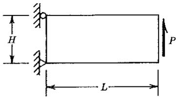Other Tests. Remarks. In the single-element test [18.17], the response of a single element to a certain loading is examined as one changes the element aspect ratio, skewness, or taper. For example, in Fig. 18.8-2, a tip-loaded cantilever beam can be repeatedly analyzed as L/H is varied from a small value to a large value. It may happen that of two competing element formulations A and B, both work well when L/H = 1 but A is much more accurate than B when L/H >> 1. Then A has proved superior in this particular test. The test is very easy to perform. When used with but one element formulation, rather than in comparing different formulations, the test provides information about element behavior that is useful in modeling. Another type of element test compares strain energies $[18.15]$ . For a prescribed deformation state, strain energy in the mathematical continuum is computed over the volume spanned by the element. Strain energy in the element is also computed by imposing nodal d.o.f. consistent with the prescribed deformation state. The two energies are compared. The test is repeated, using other deformation states. Other tests have already been noted, including the patch test (Section 4.6) and applying a finite element model to various problems whose solutions are already known. The latter test is neither definitive nor general, but one would be foolish not to use it. In testing a new element, or in becoming acquainted with an unfamiliar element, it is appropriate to use a variety of tests. No single test is likely to be decisive, except perhaps in discovering a fatally flawed element. Element behavior tends to be case-dependent, so that the ranking of competing elements is likely to be different in different test cases and is likely to depend on whether stress or displacement is taken as the indicator of quality. The ideal element, probably never to be discovered, passes patch tests, yields good results in a coarse mesh, converges rapidly with mesh refinement, is almost insensitive to shape distortion, is geometrically isotropic, has no zero- or low-energy deformation modes when assembled with other elements, can be joined to elements of different type, rests on simple theory, and is economical to formulate. 

text_image

H L P

Figure 18.8-2. Single-element model of a cantilever beam under transverse tip load. # 18.9 CONCLUDING REMARKS In this chapter we have discussed tests that can be applied to elements, to an assembly of elements, or to a set of equations. If an error or a potential difficulty is present, no single test is certain to detect it. Even if several tests are applied and passed, one should be aware that tests can detect errors but cannot prove their absence, and that a trouble-free finite element structure may not be a good model of physical reality. Physical situations in structural mechanics that make numerical error more likely include elements with great shape distortion or large aspect ratio, an element whose shear or membrane stiffness is much larger than its bending stiffness, stiff elements used to approximate a rigid region, and a very fine mesh. This is a list of guidelines rather than firm rules, as in each situation one can identify one or more special cases in which the anticipated trouble does not materialize. On most digital computers, one should use double-precision data for all constants and double-precision arithmetic for all phases of generating structural equations and solving them. Partial double precision in equation solving and double-precision solution of equations generated in single precision are dangerous practices. It is risky to generalize from a single example, yet it is interesting that practical problems with $1.5(10^{6})$ d.o.f. have been solved with good engineering accuracy. # PROBLEMS # Section 18.2 18.1 (a) Solve Eqs. 18.2-1 graphically by plotting the slope of each line and determining the intersection point. (b) Repeat part (a), using Eqs. 18.2-2 instead. 18.2 Consider the equations $x + y = 2$ and $x + 1.01y = 2.01$ . Show that the solution is sensitive in small changes in both the coefficient matrix and the vector of constants. 18.3 Show that Eq. 18.2-3 can be written in the form of Eq. 9.3-5, with $k = k_{2}$ and penalty number $\alpha = (k_{1} / k_{2}) - 1$ . What happens when $\alpha$ becomes very large? 18.4 In Eq. 18.2-4, determine the reduced coefficient $K_{22}$ produced by Gauss elimination. Show that this result predicts trouble if $\alpha$ is large. 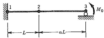18.5 The two-element beam shown is uniform, fixed at the left end, and simply supported at the right end. Show that the structural equations become ill conditioned if the scalar multiplier $\alpha$ is very small. 

text_image

1 2 3 M₀ L αL

Problem 18.5 

text_image

L P 1 2 k

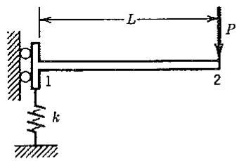
Problem 18.7 18.6 (a) Obtain Eqs. 18.2-6 by coordinate transformation of Eqs. 18.2-3. Show that large cancellation error may be present. (b) Obtain Eqs. 18.2-6 by applying coordinate transformation to [k] of the left element in Fig. 18.2-1, then assembling the two elements. 18.7 The left end of the one-element cantilever beam shown rests on a soft spring of stiffness k. Rotation is prevented at the left end. (a) Solve for the deflection of load P using $w_{1}$ , $w_{2}$ , and $\theta_{2}$ as nonzero d.o.f. Show that the equations are ill conditioned if $k << EI/L^{3}$ . (b) Form an element stiffness matrix that operates on d.o.f. $w_{1}, \theta_{1}, w_{21}$ , and $\theta_{21}$ , where $w_{21}$ and $\theta_{21}$ are the “relative” d.o.f. $w_{21} = w_{2} - (w_{1} + L\theta_{1})$ and $\theta_{21} = \theta_{2} - \theta_{1}$ . Impose one boundary condition, include the soft spring, and again solve for the deflection of load $P$ . Show that the equations are not ill conditioned. 18.8 For a general structure, how many d.o.f. can be “relative” and how many must be “absolute”? (See Problem 18.7(b) for an illustration of these terms.) # Section 18.3 18.9 (a) How small can $C(\mathbf{K})$ be? (b) What is $C(\mathbf{K})$ if $[\mathbf{K}]$ is diagonal? (c) Physically, what is implied if $C(\mathbf{K})$ is infinite? 18.10 (a) Let $k_{1} = 10k_{2}$ in Fig. 18.2-1. Compute the condition numbers of the unscaled matrix [K] and of the scaled matrix $[\mathbf{K}_s]$ . (b) Repeat part (a), now with $k_{2} = 10k_{1}$ . 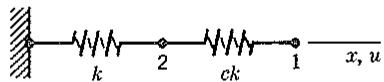18.11 (a) The two-spring system shown has d.o.f. $u_{1}$ and $u_{2}$ . For what value of scalar $c$ is the condition number of the unscaled stiffness matrix a minimum, and what is its minimum value? (b) Repeat part (a), but use the scaled stiffness matrix.  Problem 18.11 18.12 Let $\beta = 45^{\circ}$ in Fig. 18.2-3a. Compute $C(\mathbf{K})$ in terms of $\alpha$ using (a) the unscaled matrix [K], and (b) the scaled matrix $[\mathbf{K}_s]$ . 18.13 (a) Evaluate Eq. 18.3-2 for the structure shown in Fig. 18.3-1. (b) Let $AE / L = 174$ in Fig. 18.3-1a. Let a hypothetical computer retain only three significant digits per word, so that coefficients in [K] are represented as $K_{11} = -K_{12} = -K_{21} = 1040$ and $K_{22} = 1220$ . If subsequent manipulations are exact, what are the percentage errors in the computed values of $u_{1}, u_{2}$ , and $(u_{1} - u_{2}) / L$ ? Does Eq. 18.3-2 seem to apply? (c) Repeat part (b) for the problem of Fig. 18.3-1b. 18.14 Interchange the bars in Fig. 18.3-1; for example, let the left bar have stiffness 174 and the right bar have stiffness 6(174) = 1044. (a) Compute $C(\mathbf{K})$ , using first the unscaled [K] and then the scaled matrix $[\mathbf{K}_s]$ . (b) Repeat Problem 18.13(b), where now $K_{11} = -K_{12} = -K_{21} = 174$ and $K_{22} = 1220$ . 18.15 A uniform beam is modeled by a single standard beam element. What is the condition number of the scaled stiffness matrix if the beam is (a) simply supported, and (b) cantilevered? (There are two nonzero d.o.f. in each case.) 18.16 Why, in Eq. 18.3-8, can $N^{2m/n}$ be replaced by $h^{-2m}$ ? 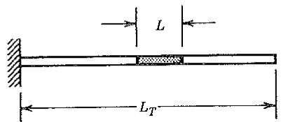(Here it is easiest to imagine that $h$ , the span of a typical element, is uniform throughout the mesh.) 18.17 The bar shown is uniform and is built of standard two-node elements. In axial vibration, its fundamental frequency $\omega_{1}$ is given by $\omega_{1}^{2} = \pi^{2}E/4L_{T}^{2}\rho$ , where $\rho$ is the mass density. (a) Let all elements have the same length $L$ . Use Eq. 18.3-9 to bound $C(\mathbf{K})$ in terms of $L_T$ and $L$ . (b) Evaluate this bound numerically, using two elements $(L = L_T / 2)$ . Also evaluate the exact $C(\mathbf{K})$ , and compare. (c) Repeat part (b), but use two unequal elements, of lengths $L$ and $2L$ , respectively. 

text_image

L L_T

Problem 18.17 # Section 18.4 18.18 (a) Write [K] for the structure shown, in which each spring has stiffness $k = 100$ . By examination of the first few steps of Gauss elimination, deduce an expression for the reduced diagonal coefficient $K_{ii}$ in terms of $k$ and $i$ . Hence, what are the diagonal decay ratios after the 99th and 100th eliminations? (b) Repeat part (a), but sequence the node numbers from right to left, so that node 1 carries load $P$ . 18.19 In each part of this problem, imagine that the analyst has forgotten to specify any displacement boundary conditions, so that the structure is unsupported. In what equation (first, second, . . ., last) of the system $[K]\{D\} = \{R\}$ will the diagonal decay test detect this trouble? (a) The train of springs in Problem 18.18. (b) The beams of Table 18.4-1. (c) A plane frame having three d.o.f. per node. (d) A solid of revolution having two d.o.f. (radial and axial) per node. (e) A plane structure having two d.o.f. per node. 18.20 Compute the diagonal decay ratio in terms of $\alpha$ for the problem described by Fig. 18.2-3a. Show that it is not large if $\beta = 0$ or if $\beta = \pi / 2$ . 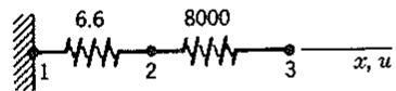18.21 With unit axial loads at nodes 2 and 3 in the structure shown, the exact 

text_image

k k k k k 1 2 99 100 101 P

Problem 18.18  Problem 18.21 structure equations are $8006.6u_{2}-8000u_{3}=1$ and $-8000u_{2}+8000u_{3}=1$ . Compute the exact values of $u_{2}$ and $u_{3}$ . Also compute approximate values under the assumption that the computer rounds numbers to only four digits after each operation of Gauss elimination. Does the accuracy loss agree with that predicted by (a) the diagonal decay ratio and (b) the condition number of [K]? 18.22 What Fortran statements should be added, and where, if a test for diagonal decay is to be incorporated in the equation solver provided in Fig. B.2-3? # Section 18.5 18.23 Consider the two equations $1.78u_{1} + 1.06u_{2} = 2.88$ and $0.94u_{1} + 0.56u_{2} = 1.52$ . What residual vector $\{\Delta \mathbf{R}\}$ is given by the approximate solution $u_{1} = 1.88$ , $u_{2} = -0.44$ , and what is $e$ of Eq. 18.5-2? What is the exact solution? Are the equations ill conditioned? 18.24 Consider the ill-conditioned equations $u_{1} + u_{2} = 2$ , $u_{1} + 1.0001u_{2} = 2.0001$ . What residuals and what e are given by the approximate solution $u_{1} = 2.0$ , $u_{2} = 0.0$ , and by the approximate solution $u_{1} = u_{2} = 1.1$ ? Which of the two approximate solutions is most nearly correct? 18.25 A linear spring of stiffness 28 N/m is loaded by a 0.5-N force. Using the approximate value $k^{-1} \approx 0.040$ m/N, we compute the approximate displacement $u \approx 0.020$ m. Improve this result by the iterative method, associated with Eq. 18.5-1, using the correct k and the approximate $k^{-1}$ . 18.26 Consider the two equations $(u_{1} / 3) - (u_{2} / 3) = 1$ and $-(u_{1} / 3) + (7u_{2} / 12) = 0$ . Let the stiffness matrix and its inverse be approximated as $$ [ \mathbf {K} ] \approx \left[ \begin{array}{c c} 0. 3 & - 0. 3 \\ - 0. 3 & 0. 5 \end{array} \right] \quad \text { and } \quad [ \mathbf {K} ] ^ {- 1} \approx \left[ \begin{array}{c c} 8. 0 & 5. 0 \\ 5. 0 & 5. 0 \end{array} \right] $$ (a) Use the foregoing approximate matrices in 18.5-1. Apply three cycles of iterative improvement. Do displacements $u_{1}$ and $u_{2}$ appear to be converging toward correct values? (b) Use the approximate $[\mathbf{K}]^{-1}$ to compute $\{\Delta \mathbf{D}\} = [\mathbf{K}]^{-1}\{\Delta \mathbf{R}\}$ but the correct [K] to compute $\{\Delta \mathbf{R}\}$ . Again apply three cycles of iterative improvement and assess the results. 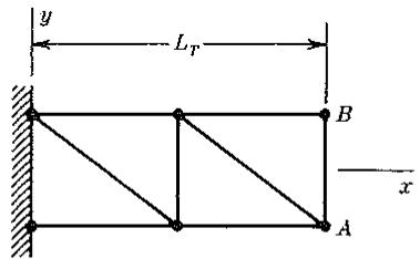18.27 The cantilever beam shown is built of four constant-strain triangles (described in Chapter 5). For what loadings at nodes A and B will computed results be exact? For which of these loadings will residuals be essentially zero? For each loading plot the qualitative variation of $\sigma_{x}$ along the x axis, according to your expectation of the finite element results. 

text_image

y Lr B x A

Problem 18.27 # Section 18.6 18.28 For the bar problem of Fig. 18.6-1, show that the finite element solution yields exact displacements at the nodes when $A$ and $E$ are constant and the load integral, $\int [\mathbf{N}]^T q dx$ , is evaluated consistently over length $h_i$ of each element. Assume that $q = q(x)$ is a continuous function for $x_i \leq x \leq x_{i+1}$ . Suggestion: First show that the exact solution is $$ A E u (x) = - \int_ {0} ^ {x} \int_ {0} ^ {s} q (\ell) d \ell d s + x \int_ {0} ^ {L _ {T}} q (\ell) d \ell \tag {a} $$ Then evaluate the nodal load vector consistently. Integrate each entry by parts to show that the ith entry of the nodal load vector is $$ \begin{array}{l} \int_ {0} ^ {h _ {i - 1}} q (x + x _ {i - 1}) d x - \frac {1}{h _ {i - 1}} \int_ {0} ^ {h _ {i - 1}} \int_ {0} ^ {x} q (s + x _ {i - 1}) d s d x \\ + \frac {1}{h _ {i}} \int_ {0} ^ {h _ {i}} \int_ {0} ^ {x} q (s + x _ {i}) d s d x \tag {b} \\ \end{array} $$ The last integral is absent in the load at $L_{T}$ . Since the response at the nodes, $x_{i}$ , to given nodal loads is exact for bar elements, deduce the response to these nodal loads exactly, and show that the result coincides with Eq. (a) at the nodes. 18.29 From Problem 18.28 we may deduce that the error function $e(x)$ defined in Eq. 18.6-2 has the expansion given in Eq. 18.6-3 on element $i$ . Show that $e'(x_i) = (h_i/2)u''(\bar{x})$ for an $\bar{x}$ in the $i$ th element. Suggestion: From Eq. (a) and Eq. 18.6-2, we may easily deduce that $$ e ^ {\prime} (x _ {i}) = \frac {1}{A E} \int_ {x _ {i}} ^ {L _ {T}} q (x) d x - \frac {u _ {i + 1} - u _ {i}}{h _ {i}} \tag {c} $$ Express $u_{i+1}$ and $u_{i}$ using Eq. (a), since these values have been shown to be exact in problem 18.28. Apply the mean value theorem for integrals to the resulting expression. 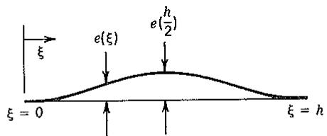18.30 If a uniform beam carries a smooth and continuous distributed lateral load, the standard beam element yields exact values of nodal displacements and rotations. Therefore, over one element, error $e(x)$ in lateral displacement has the appearance shown. A Taylor series analysis shows that the leading term in an expansion like Eq. 18.6-3 for $e(x)$ is $\frac{1}{2}(x - x_i)^2 e''(\overline{x})$ for an $\overline{x}$ in the element. Show that $e(x) = O(h^4)$ . Suggestion: Use the $N_i$ of Fig. 3.13-2, and show that if $u(0), u'(0), u(h)$ , and $u'(h)$ are exact, then $e(h/2) = O(h^4)$ and $e'(h/2) = O(h^3)$ on the element. Then 

text_image

ξ e(ξ) e(h/2) ξ = 0 ξ = h

Problem 18.30