text_image

223,000 lb-in. 3700 lb 4990 lb 120 in. 376,000 lb-in. 376,000 lb 4990 lb 3700 lb x̂ y ẑ

(a) 

text_image

5010 lb 2 3700 lb 3700 lb 120 in. 223,000 lb-in. 221,000 lb-in. 3 5010 lb 3

(b) 

text_image

3700 lb 226,000 lb-in. 5010 lb x̂ ŷ 120 in. 5010 lb 375,000 lb-in. 3700 lb

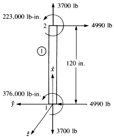
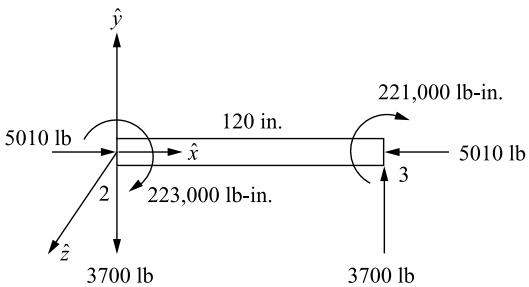
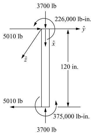
（c) Figure 5–5 Free-body diagrams of (a) element 1, (b) element 2, and (c) element 3 Considering the free body of element 1, the equilibrium equations are $$ \sum F _ {\hat {x}}: - 4 9 9 0 + 4 9 9 0 = 0 $$ $$ \sum F _ {\hat {y}}: - 3 7 0 0 + 3 7 0 0 = 0 $$ $$ \sum M _ {2}: 3 7 6, 0 0 0 + 2 2 3, 0 0 0 - 4 9 9 0 (1 2 0 \text { in. }) \cong 0 $$ Considering moment equilibrium at node 2, we see from Eqs. (5.2.12a) and (5.2.12b) that on element 1, $\hat { m } _ { 2 } = 2 2 3 , 0 0 0$ lb-in., and the opposite value, -223,000 lb-in., occurs on element 2. Similarly, moment equilibrium is satisfied at node 3, as m^3 from elements 2 and 3 add to the 5000 lb-in. applied moment. That is, from Eqs. (5.2.12a) and (5.2.12b) we have $$ - 2 2 1, 0 0 0 + 2 2 6, 0 0 0 = 5 0 0 0 \mathrm{lb-in}. $$ # Example 5.2 To illustrate the procedure for solving frames subjected to distributed loads, solve the rigid plane frame shown in Figure 5–6. The frame is fixed at nodes 1 and 3 and subjected to a uniformly distributed load of 1000 lb/ft applied downward over element 2. The global-coordinate axes have been established at node 1. The element lengths are shown in the figure. Let $E = 3 0 \times 1 0 ^ { 6 } \mathrm { p s i } , A = 1 0 0 \mathrm { i n } ^ { 2 } .$ , and $I = 1 0 0 0 \mathrm { i n } ^ { 4 }$ for both elements of the frame. We begin by replacing the distributed load acting on element 2 by nodal forces and moments acting at nodes 2 and 3. Using Eqs. (4.4.5)–(4.4.7) (or Appendix D), the equivalent nodal forces and moments are calculated as $$ f _ {2 y} = - \frac {w L}{2} = - \frac {(1 0 0 0) 4 0}{2} = - 2 0, 0 0 0 \mathrm{lb} = - 2 0 \mathrm{kip} \tag {5.2.13} $$ $$ m _ {2} = - \frac {w L ^ {2}}{1 2} = - \frac {(1 0 0 0) 4 0 ^ {2}}{1 2} = - 1 3 3, 3 3 3 \mathrm{lb-ft} = - 1 6 0 0 \mathrm{k-in}. 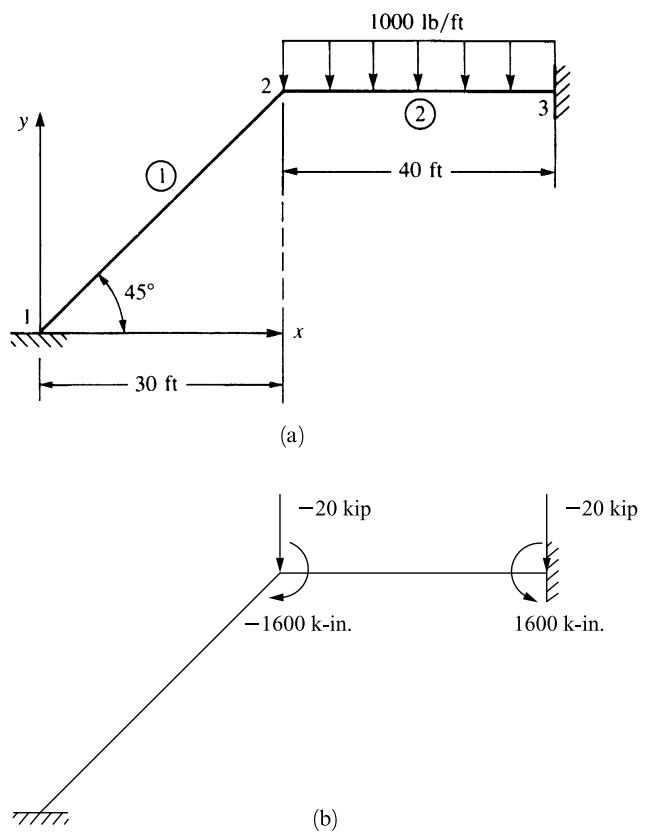$$  Figure 5–6 (a) Plane frame for analysis and (b) equivalent nodal forces on frame $$ f _ {3 y} = - \frac {w L}{2} = - \frac {(1 0 0 0) 4 0}{2} = - 2 0, 0 0 0 \mathrm{lb} = - 2 0 \mathrm{kip} $$ $$ m _ {3} = \frac {w L ^ {2}}{1 2} = \frac {(1 0 0 0) 4 0 ^ {2}}{1 2} = 1 3 3, 3 3 3 \mathrm{lb-ft} = 1 6 0 0 \mathrm{k-in}. $$ We then use Eq. (5.1.11), to determine each element stiffness matrix: # Element 1 $$ \theta^ {(1)} = 4 5 ^ {\circ} \quad C = 0. 7 0 7 \quad S = 0. 7 0 7 \quad L ^ {(1)} = 4 2. 4 \mathrm{ft} = 5 0 9. 0 \mathrm{in}. $$ $$ \frac {E}{L} = \frac {3 0 \times 1 0 ^ {3}}{5 0 9} = 5 8. 9 3 $$ $$ \underline {{k}} ^ {(1)} = 5 8. 9 3 \left[ \begin{array}{c c c} 5 0. 0 2 & 4 9. 9 8 & 8. 3 3 \\ 4 9. 9 8 & 5 0. 0 2 & - 8. 3 3 \\ 8. 3 3 & - 8. 3 3 & 4 0 0 0 \end{array} \right] \frac {\mathrm{kip}}{\mathrm{in.}} \tag {5.2.14} $$ Simplifying Eq. (5.2.14), we obtain $$ \underline {{k}} ^ {(1)} = \left[ \begin{array}{c c c} d _ {2 x} & d _ {2 y} & \phi_ {2} \\ 2 9 4 8 & 2 9 4 5 & 4 9 1 \\ 2 9 4 5 & 2 9 4 8 & - 4 9 1 \\ 4 9 1 & - 4 9 1 & 2 3 5, 7 0 0 \end{array} \right] \frac {\mathrm{kip}}{\text { in. }} \tag {5.2.15} $$ where only the parts of the stiffness matrix associated with degrees of freedom at node 2 are included because node 1 is fixed. # Element 2 $$ \theta^ {(2)} = 0 ^ {\circ} \quad C = 1 \quad S = 0 \quad L ^ {(2)} = 4 0 \mathrm{ft} = 4 8 0 \mathrm{in}. $$ $$ \frac {E}{L} = \frac {3 0 \times 1 0 ^ {3}}{4 8 0} = 6 2. 5 0 $$ $$ \underline {{k}} ^ {(2)} = 6 2. 5 0 \left[ \begin{array}{c c c} 1 0 0 & 0 & 0 \\ 0 & 0. 0 5 2 & 1 2. 5 \\ 0 & 1 2. 5 & 4 0 0 0 \end{array} \right] \frac {\mathrm{kip}}{\text { in. }} \tag {5.2.16} $$ Simplifying Eq. (5.2.16), we obtain $$ \underline {{k}} ^ {(2)} = \left[ \begin{array}{c c c} d _ {2 x} & d _ {2 y} & \phi_ {2} \\ 6 2 5 0 & 0 & 0 \\ 0 & 3. 2 5 & 7 8 1. 2 5 \\ 0 & 7 8 1. 2 5 & 2 5 0, 0 0 0 \end{array} \right] \frac {\mathrm{kip}}{\mathrm{in.}} \tag {5.2.17} $$ where, again, only the parts of the stiffness matrix associated with degrees of freedom at node 2 are included because node 3 is fixed. On superimposing the stiffness matrices of the elements, using Eqs. (5.2.15) and (5.2.17), and using Eq. (5.2.13) for the nodal forces and moments only at node 2 (because the structure is fixed at node 3), we have $$ \left\{ \begin{array}{l} F _ {2 x} = 0 \\ F _ {2 y} = - 2 0 \\ M _ {2} = - 1 6 0 0 \end{array} \right\} = \left[ \begin{array}{c c c} 9 1 9 8 & 2 9 4 5 & 4 9 1 \\ 2 9 4 5 & 2 9 5 1 & 2 9 0 \\ 4 9 1 & 2 9 0 & 4 8 5, 7 0 0 \end{array} \right] \left\{ \begin{array}{l} d _ {2 x} \\ d _ {2 y} \\ \phi_ {2} \end{array} \right\} \tag {5.2.18} $$ Solving Eq. (5.2.18) for the displacements and the rotation at node 2, we obtain $$ \left\{ \begin{array}{l} d _ {2 x} \\ d _ {2 y} \\ \phi_ {2} \end{array} \right\} = \left\{ \begin{array}{c} 0. 0 0 3 3 \text { in. } \\ - 0. 0 0 9 7 \text { in. } \\ - 0. 0 0 3 3 \text { rad } \end{array} \right\} \tag {5.2.19} $$ The results indicate that node 2 moves to the right $( d _ { 2 x } = 0 . 0 0 3 3$ in.) and down $( d _ { 2 y } = - 0 . 0 0 9 7 \mathrm { i n . } )$ and the rotation of the joint is clockwise $( \phi _ { 2 } = - 0 . 0 0 3 3 ~ \mathrm { r a d } )$ . The local forces in each element can now be determined. The procedure for elements that are subjected to a distributed load must be applied to element 2. Recall that the local forces are given by $\underline { { \hat { f } } } = \underline { { \hat { k } } } \underline { { T } } \underline { { d } } .$ . For element 1, we then have $$ \underline {{{T}}} \underline {{{d}}} = \left[ \begin{array}{c c c c c c} 0. 7 0 7 & 0. 7 0 7 & 0 & 0 & 0 & 0 \\ - 0. 7 0 7 & 0. 7 0 7 & 0 & 0 & 0 & 0 \\ 0 & 0 & 1 & 0 & 0 & 0 \\ 0 & 0 & 0 & 0. 7 0 7 & 0. 7 0 7 & 0 \\ 0 & 0 & 0 & - 0. 7 0 7 & 0. 7 0 7 & 0 \\ 0 & 0 & 0 & 0 & 0 & 1 \end{array} \right] \left\{ \begin{array}{l} 0 \\ 0 \\ 0 \\ 0. 0 0 3 3 \\ - 0. 0 0 9 7 \\ - 0. 0 0 3 3 \end{array} \right\} \tag {5.2.20} $$ Simplifying Eq. (5.2.20) yields $$ \underline {{T}} \underline {{d}} = \left\{ \begin{array}{c} 0 \\ 0 \\ 0 \\ - 0. 0 0 4 5 2 \\ - 0. 0 0 9 2 \\ - 0. 0 0 3 3 \end{array} \right\} \tag {5.2.21} $$ Using Eq. (5.2.21) and Eq. (5.1.8) for $\underline { { \hat { k } } } ,$ , we obtain $$ \left\{ \begin{array}{l} \hat {f} _ {1 x} \\ \hat {f} _ {1 y} \\ \hat {m} _ {1} \\ \hat {f} _ {2 x} \\ \hat {f} _ {2 y} \\ \hat {m} _ {2} \end{array} \right\} = \left[ \begin{array}{c c c c c c} 5 8 9 3 & 0 & 0 & - 5 8 9 3 & 0 & 0 \\ & 2. 7 3 0 & 6 9 4. 8 & 0 & - 2. 7 3 0 & 6 9 4. 8 \\ & & 1 1 7, 9 0 0 & 0 & - 6 9 4. 8 & 1 1 7, 9 0 0 \\ & & & 5 8 9 3 & 0 & 0 \\ & & & & 2. 7 3 0 & - 6 9 4. 8 \\ \text {Symmetry} & & & & & 2 3 5, 8 0 0 \end{array} \right] \left\{ \begin{array}{l} 0 \\ 0 \\ 0 \\ - 0. 0 0 4 5 2 \\ - 0. 0 0 9 2 \\ - 0. 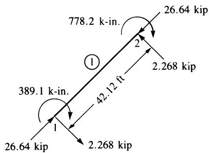0 0 3 3 \end{array} \right\} \tag {5.2.22} $$ Simplifying Eq. (5.2.22) yields the local forces in element 1 as $$ \hat {f} _ {1 x} = 2 6. 6 4 \text {kip} \quad \hat {f} _ {1 y} = - 2. 2 6 8 \text {kip} \quad \hat {m} _ {1 x} = - 3 8 9. 1 \text {k - in}. \tag {5.2.23} $$ $$ \hat {f} _ {2 x} = - 2 6. 6 4 \mathrm{kip} \quad \hat {f} _ {2 y} = 2. 2 6 8 \mathrm{kip} \quad \hat {m} _ {2 x} = - 7 7 8. 2 \mathrm{k-in}. $$ For element 2, the local forces are given by Eq. (4.4.11) because a distributed load is acting on the element. From Eqs. (5.1.10) and (5.2.19), we then have $$ \underline {{{T}}} \underline {{{d}}} = \left[ \begin{array}{c c c c c c} 1 & 0 & 0 & 0 & 0 & 0 \\ 0 & 1 & 0 & 0 & 0 & 0 \\ 0 & 0 & 1 & 0 & 0 & 0 \\ 0 & 0 & 0 & 1 & 0 & 0 \\ 0 & 0 & 0 & 0 & 1 & 0 \\ 0 & 0 & 0 & 0 & 0 & 1 \end{array} \right] \left\{ \begin{array}{c} 0. 0 0 3 3 \\ - 0. 0 0 9 7 \\ - 0. 0 0 3 3 \\ 0 \\ 0 \\ 0 \end{array} \right\} \tag {5.2.24} $$ Simplifying Eq. (5.2.24), we obtain $$ \left\{ \begin{array}{c} 0. 0 0 3 3 \\ - 0. 0 0 9 7 \\ - 0. 0 0 3 3 \\ 0 \\ 0 \\ 0 \end{array} \right\} \tag {5.2.25} $$ Using Eq. (5.2.25) and Eq. (5.1.8) for $\underline { { \hat { k } } } ,$ we have $$ \hat {\underline {{k}}} \hat {\underline {{d}}} = \hat {\underline {{k}}} \underline {{T}} \underline {{d}} = \left[ \begin{array}{c c c c c c} 6 2 5 0 & 0 & 0 & - 6 2 5 0 & 0 & 0 \\ & 3. 2 5 & 7 8 1. 1 & 0 & - 3. 2 5 & 7 8 1. 1 \\ & & 2 5 0, 0 0 0 & 0 & - 7 8 1. 1 & 1 2 5, 0 0 0 \\ & & & 6 2 5 0 & 0 & 0 \\ & & & & 3. 2 5 & - 7 8 1. 1 \\ \text {Symmetry} & & & & & 2 5 0, 0 0 0 \end{array} \right] \left\{ \begin{array}{c} 0. 0 0 3 3 \\ - 0. 0 0 9 7 \\ - 0. 0 0 3 3 \\ 0 \\ 0 \\ 0 \end{array} \right\} \tag {5.2.26} $$ Simplifying Eq. (5.2.26) yields $$ \underline {{\hat {k}}} \underline {{\hat {d}}} = \left\{ \begin{array}{r} 2 0. 6 3 \\ - 2. 5 8 \\ - 8 3 2. 5 7 \\ - 2 0. 6 3 \\ 2. 5 8 \\ - 4 1 2. 5 0 \end{array} \right\} \tag {5.2.27} $$ 

text_image

778.2 k-in. 26.64 kip 2 2.268 kip 389.1 k-in. 42.12 ft 2.268 kip 26.64 kip 1


text_image

20.63 kip 767.4 k-in. 1.00 k/ft 2013 k-in. 20.63 kip 17.42 kip 40 ft 22.58 kip 2 ② 3

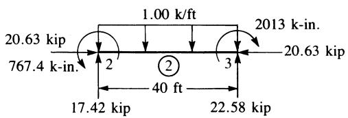
Figure 5–7 Free-body diagrams of elements 1 and 2 To obtain the actual element local nodal forces, we apply Eq. (4.4.11); that is, we must subtract the equivalent nodal forces [Eqs. (5.2.13)] from Eq. (5.2.27) to yield $$ \left\{ \begin{array}{l} \hat {f} _ {2 x} \\ \hat {f} _ {2 y} \\ \hat {m} _ {2} \\ \hat {f} _ {3 x} \\ \hat {f} _ {3 y} \\ \hat {m} _ {3} \end{array} \right\} = \left\{ \begin{array}{c} 2 0. 6 3 \\ - 2. 5 8 \\ - 8 3 2. 5 7 \\ - 2 0. 6 3 \\ 2. 5 8 \\ - 4 1 2. 5 0 \end{array} \right\} - \left\{ \begin{array}{c} 0 \\ - 2 0 \\ - 1 6 0 0 \\ 0 \\ - 2 0 \\ 1 6 0 0 \end{array} \right\} \tag {5.2.28} $$ Simplifying Eq. (5.2.28), we obtain $$ \hat {f} _ {2 x} = 2 0. 6 3 \mathrm{kip} \quad \hat {f} _ {2 y} = 1 7. 4 2 \mathrm{kip} \quad \hat {m} _ {2} = 7 6 7. 4 \mathrm{k} - \text {in}. \tag {5.2.29} $$ $$ \hat {f} _ {3 x} = - 2 0. 6 3 \mathrm{kip} \quad \hat {f} _ {3 y} = 2 2. 5 8 \mathrm{kip} \quad \hat {m} _ {3} = - 2 0 1 3 \mathrm{k-in}. $$ Using Eqs. (5.2.23) and (5.2.29) for the local forces in each element, we can construct the free-body diagram for each element, as shown in Figure 5–7. From the freebody diagrams, one can confirm the equilibrium of each element, the total frame, and joint 2 as desired. 9 In Example 5.3, we will illustrate the equivalent joint force replacement method for a frame subjected to a load acting on an element instead of at one of the joints of the structure. Since no distributed loads are present, the point of application of the concentrated load could be treated as an extra joint in the analysis, and we could solve the problem in the same manner as Example 5.1. This approach has the disadvantage of increasing the total number of joints, as well as the size of the total structure stiffness matrix K. For small structures solved by computer, this does not pose a problem. However, for very large structures, this might reduce the maximum size of the structure that could be analyzed. Certainly, this additional node greatly increases the longhand solution time for the structure. Hence, we will illustrate a standard procedure based on the concept of equivalent joint forces applied to the case of concentrated loads. We will again use Appendix D. 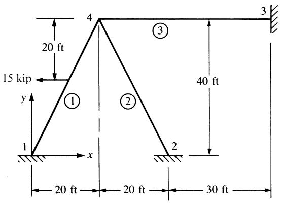Solve the frame shown in Figure 5–8(a). The frame consists of the three elements shown and is subjected to a 15-kip horizontal load applied at midlength of element 1. Nodes 1, 2, and 3 are fixed, and the dimensions are shown in the figure. Let $E = 3 0 \times 1 0 ^ { 6 } \ \mathrm { p s i } , I = 8 0 0 \ \mathrm { i n } ^ { 4 } .$ , and $A = 8 \mathrm { i n } ^ { 2 }$ for all elements. 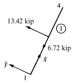1. We first express the applied load in the element 1 local coordinate system (here x^ is directed from node 1 to node 4). This is shown in Figure 5–8(b). 

text_image

20 ft 15 kip ① ② ③ 40 ft 1 2 3 20 ft 20 ft 30 ft

(a） Rigid frame 

text_image

13.42 kip 6.72 kip x̂ 1 4 ① ŷ

(b）Applied load expressed in element 1 localcoordinate system 

text_image

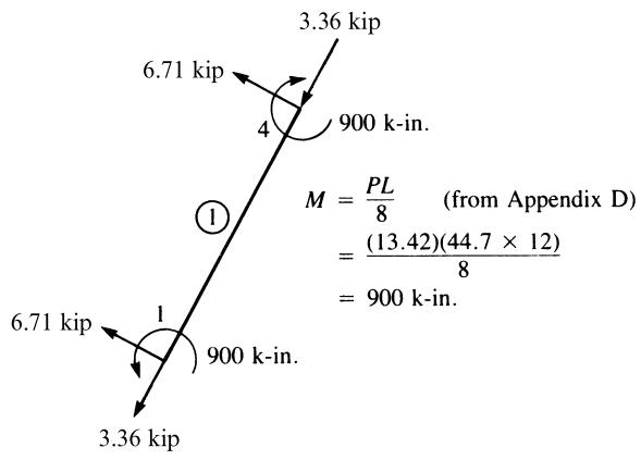
3.36 kip 6.71 kip 4 900 k-in. M = PL/8 (from Appendix D) = (13.42)(44.7 × 12)/8 = 900 k-in. 6.71 kip 1 900 k-in. 3.36 kip

(c）Equivalent joint forces expressed in local-coordinate system 

text_image

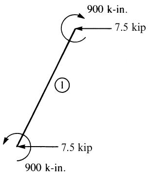
900 k-in. 7.5 kip ① 7.5 kip 900 k-in.

(d） Final equivalent joint forces expressed in global-coordinate system Figure 5–8 Rigid frame with a load applied on an element 2. Next, we determine the equivalent joint forces at each end of element 1, using the table in Appendix D. (These forces are of opposite sign from what are traditionally known as fixed-end forces in classical structural analysis theory [1].) These equivalent forces (and moments) are shown in Figure 5–8(c). 3. We then transform the equivalent joint forces from the present localcoordinate-system forces into the global-coordinate-system forces, using the equation $\underline { { f } } = \underline { { T } } ^ { T } \underline { { \hat { f } } }$ , where T is defined by Eq. (5.1.10). These global joint forces are shown in Figure 5–8(d). 4. Then we analyze the structure in Figure 5–8(d), using the equivalent joint forces (plus actual joint forces, if any) in the usual manner. 5. We obtain the final internal forces developed at the ends of each element that has an applied load (here element 1 only) by subtracting step 2 joint forces from step 4 joint forces; that is, Eq. (4.4.11) is applied locally to all elements that originally had loads acting on them. The solution of the structure as shown in Figure 5–8(d) now follows. Using Eq. (5.1.11), we obtain the global stiffness matrix for each element. # Element 1 For element 1, the angle between the global x and the local x^ axes is 63:43 because x^ is assumed to be directed from node 1 to node 4. Therefore, $$ C = \cos 6 3. 4 3 ^ {\circ} = \frac {x _ {4} - x _ {1}}{L ^ {(1)}} = \frac {2 0 - 0}{4 4 . 7} = 0. 4 4 7 $$ $$ S = \sin 6 3. 4 3 ^ {\circ} = \frac {y _ {4} - y _ {1}}{L ^ {(1)}} = \frac {4 0 - 0}{4 4 . 7} = 0. 8 9 5 $$ $$ \frac {1 2 I}{L ^ {2}} = \frac {1 2 (8 0 0)}{(4 4 . 7 \times 1 2) ^ {2}} = 0. 0 3 3 4 \quad \frac {6 I}{L} = \frac {6 (8 0 0)}{4 4 . 7 \times 1 2} = 8. 9 5 $$ $$ \frac {E}{L} = \frac {3 0 \times 1 0 ^ {3}}{4 4 . 7 \times 1 2} = 5 5. 9 $$ Using the preceding results in Eq. (5.1.11) for k, we obtain $$ \underline {{k}} ^ {(1)} = \left[ \begin{array}{c c c} d _ {4 x} & d _ {4 y} & \phi_ {4} \\ 9 0. 9 & 1 7 8 & 4 4 8 \\ 1 7 8 & 3 5 9 & - 2 2 4 \\ 4 4 8 & - 2 2 4 & 1 7 9, 0 0 0 \end{array} \right] \tag {5.2.30} $$ where only the parts of the stiffness matrix associated with degrees of freedom at node 4 are included because node 1 is fixed and, hence, not needed in the solution for the nodal displacements. # Element 3 For element 3, the angle between x and x^ is zero because x^ is directed from node 4 to node 3. Therefore, $$ C = 1 \quad S = 0 \quad \frac {1 2 I}{L ^ {2}} = \frac {1 2 (8 0 0)}{(5 0 \times 1 2) ^ {2}} = 0. 0 2 6 7 $$ $$ \frac {6 I}{L} = \frac {6 (8 0 0)}{5 0 \times 1 2} = 8. 0 0 \quad \frac {E}{L} = \frac {3 0 \times 1 0 ^ {3}}{5 0 \times 1 2} = 5 0 $$ Substituting these results into $\underline { { k } } ,$ we obtain $$ \underline {{k}} ^ {(3)} = \left[ \begin{array}{c c c} d _ {4 x} & d _ {4 y} & \phi_ {4} \\ 4 0 0 & 0 & 0 \\ 0 & 1. 3 3 4 & 4 0 0 \\ 0 & 4 0 0 & 1 6 0, 0 0 0 \end{array} \right] \tag {5.2.31} $$ since node 3 is fixed. # Element 2 For element 2, the angle between x and x^ is $1 1 6 . 5 7 ^ { \circ }$ because x^ is directed from node 2 to node 4. Therefore, $$ C = \frac {2 0 - 4 0}{4 4 . 7} = - 0. 4 4 7 \quad S = \frac {4 0 - 0}{4 4 . 7} = 0. 8 9 5 $$ $$ \frac {1 2 I}{L ^ {2}} = 0. 0 3 3 4 \quad \frac {6 I}{L} = 8. 9 5 \quad \frac {E}{L} = 5 5. 9 $$ since element 2 has the same properties as element 1. Substituting these results into k, we obtain $$ \underline {{k}} ^ {(2)} = \left[ \begin{array}{c c c} d _ {4 x} & d _ {4 y} & \phi_ {4} \\ 9 0. 9 & - 1 7 8 & 4 4 8 \\ - 1 7 8 & 3 5 9 & 2 2 4 \\ 4 4 8 & 2 2 4 & 1 7 9, 0 0 0 \end{array} \right] \tag {5.2.32} $$ since node 2 is fixed. On superimposing the stiffness matrices given by Eqs. (5.2.30), (5.2.31), and (5.2.32), and using the nodal forces given in Figure 5–8(d) at node 4 only, we have $$ \left\{ \begin{array}{c} - 7. 5 0 \mathrm{kip} \\ 0 \\ - 9 0 0 \mathrm{k} - \text { in. } \end{array} \right\} = \left[ \begin{array}{c c c} 5 8 2 & 0 & 8 9 6 \\ 0 & 7 1 9 & 4 0 0 \\ 8 9 6 & 4 0 0 & 5 1 8, 0 0 0 \end{array} \right] \left\{ \begin{array}{c} d _ {4 x} \\ d _ {4 y} \\ \phi_ {4} \end{array} \right\} \tag {5.2.33} $$ Simultaneously solving the three equations in Eq. (5.2.33), we obtain $$ d _ {4 x} = - 0. 0 1 0 3 \text { in. } $$ $$ d _ {4 y} = 0. 0 0 0 9 5 6 \text { in. } \tag {5.2.34} $$ $$ \phi_ {4} = - 0. 0 0 1 7 2 \mathrm{rad} $$ Next, we determine the element forces by again using $\underline { { \hat { f } } } = \underline { { \hat { k } } } \underline { { T } } \underline { { d } } .$ . In general, we have $$ \underline {{T}} \underline {{d}} = \left[ \begin{array}{c c c c c c} C & S & 0 & 0 & 0 & 0 \\ - S & C & 0 & 0 & 0 & 0 \\ 0 & 0 & 1 & 0 & 0 & 0 \\ 0 & 0 & 0 & C & S & 0 \\ 0 & 0 & 0 & - S & C & 0 \\ 0 & 0 & 0 & 0 & 0 & 1 \end{array} \right] \left\{ \begin{array}{c} d _ {i x} \\ d _ {i y} \\ \phi_ {i} \\ d _ {j x} \\ d _ {j y} \\ \phi_ {j} \end{array} \right\} $$ Thus, the preceding matrix multiplication yields $$ \underline {{{T}}} \underline {{{d}}} = \left\{ \begin{array}{c} C d _ {i x} + S d _ {i y} \\ - S d _ {i x} + C d _ {i y} \\ \phi_ {i} \\ C d _ {j x} + S d _ {j y} \\ - S d _ {j x} + C d _ {j y} \\ \phi_ {j} \end{array} \right\} \tag {5.2.35} $$ # Element 1 $$ \underline {{T d}} = \left\{ \begin{array}{c} 0 \\ 0 \\ 0 \\ (0. 4 4 7) (- 0. 0 1 0 3) + (0. 8 9 5) (0. 0 0 0 9 5 6) \\ (- 0. 8 9 5) (- 0. 0 1 0 3) + (0. 4 4 7) (0. 0 0 0 9 5 6) \\ - 0. 0 0 1 7 2 \end{array} \right\} = \left\{ \begin{array}{c} 0 \\ 0 \\ 0 \\ - 0. 0 0 3 7 4 \\ 0. 0 0 9 6 3 \\ - 0. 0 0 1 7 2 \end{array} \right\} \tag {5.2.36} $$ Using Eq. (5.1.8) for $\underline { { \hat { k } } }$ and Eq. (5.2.36), we obtain $$ \hat {\underline {{k}}} \underline {{T}} \underline {{d}} = \left[ \begin{array}{c c c c c c} 4 4 7 & 0 & 0 & - 4 4 7 & 0 & 0 \\ 0 & 1. 8 6 8 & 5 0 0. 5 & 0 & - 1. 8 6 8 & 5 0 0. 5 \\ 0 & 5 0 0. 5 & 1 7 9, 0 0 0 & 0 & - 5 0 0. 5 & 8 9, 4 9 0 \\ - 4 4 7 & 0 & 0 & 4 4 7 & 0 & 0 \\ 0 & - 1. 8 6 8 & - 5 0 0. 5 & 0 & 1. 8 6 8 & - 5 0 0. 5 \\ 0 & 5 0 0. 5 & 8 9, 4 9 0 & 0 & - 5 0 0. 5 & 1 7 9, 0 0 0 \end{array} \right] \times \left\{ \begin{array}{c} 0 \\ 0 \\ 0 \\ - 0. 0 0 3 7 4 \\ 0. 0 0 9 6 3 \\ - 0. 0 0 1 7 2 \end{array} \right\} \tag {5.2.37} $$ These values are now called effective nodal forces. Multiplying the matrices of Eq. (5.2.37) and using Eq. (4.4.11) to subtract the equivalent nodal forces in local coordinates for the element shown in Figure $5 \mathrm { - } 8 ( \mathrm { c } )$ , we obtain the final nodal forces in