$\alpha _ { i } , \alpha _ { j } , \ldots , \gamma _ { m } ,$ and unknown nodal displacements $u _ { i } , u _ { j }$ , and $u _ { m }$ . Beginning with Eqs. (6.2.2) expressed in matrix form, we have $$ \{u \} = \left[ \begin{array}{l l l} 1 & x & y \end{array} \right] \left\{ \begin{array}{l} a _ {1} \\ a _ {2} \\ a _ {3} \end{array} \right\} \tag {6.2.13} $$ Substituting Eq. (6.2.11) into Eq. (6.2.13), we obtain $$ \{u \} = \frac {1}{2 A} [ 1 \quad x \quad y ] \left[ \begin{array}{c c c} \alpha_ {i} & \alpha_ {j} & \alpha_ {m} \\ \beta_ {i} & \beta_ {j} & \beta_ {m} \\ \gamma_ {i} & \gamma_ {j} & \gamma_ {m} \end{array} \right] \left\{ \begin{array}{l} u _ {i} \\ u _ {j} \\ u _ {m} \end{array} \right\} \tag {6.2.14} $$ Expanding Eq. (6.2.14), we have $$ \{u \} = \frac {1}{2 A} [ 1 \quad x \quad y ] \left\{ \begin{array}{l} \alpha_ {i} u _ {i} + \alpha_ {j} u _ {j} + \alpha_ {m} u _ {m} \\ \beta_ {i} u _ {i} + \beta_ {j} u _ {j} + \beta_ {m} u _ {m} \\ \gamma_ {i} u _ {i} + \gamma_ {j} u _ {j} + \gamma_ {m} u _ {m} \end{array} \right\} \tag {6.2.15} $$ Multiplying the two matrices in Eq. (6.2.15) and rearranging, we obtain $$ u (x, y) = \frac {1}{2 A} \left\{\left(\alpha_ {i} + \beta_ {i} x + \gamma_ {i} y\right) u _ {i} + \left(\alpha_ {j} + \beta_ {j} x + \gamma_ {j} y\right) u _ {j} + \left(\alpha_ {m} + \beta_ {m} x + \gamma_ {m} y\right) u _ {m} \right\} \tag {6.2.16} $$ Similarly, replacing $u _ { i }$ by $v _ { i } , u _ { j }$ by $v _ { j } ,$ , and $u _ { m }$ by $v _ { m }$ in Eq. (6.2.16), we have the y displacement given by $$ v (x, y) = \frac {1}{2 A} \left\{\left(\alpha_ {i} + \beta_ {i} x + \gamma_ {i} y\right) v _ {i} + \left(\alpha_ {j} + \beta_ {j} x + \gamma_ {j} y\right) v _ {j} + \left(\alpha_ {m} + \beta_ {m} x + \gamma_ {m} y\right) v _ {m} \right\} \tag {6.2.17} $$ To express Eqs. (6.2.16) and (6.2.17) for u and v in simpler form, we define $$ N _ {i} = \frac {1}{2 A} (\alpha_ {i} + \beta_ {i} x + \gamma_ {i} y) $$ $$ N _ {j} = \frac {1}{2 A} (\alpha_ {j} + \beta_ {j} x + \gamma_ {j} y) \tag {6.2.18} $$ $$ N _ {m} = \frac {1}{2 A} (\alpha_ {m} + \beta_ {m} x + \gamma_ {m} y) $$ Thus, using Eqs. (6.2.18), we can rewrite Eqs. (6.2.16) and (6.2.17) as $$ u (x, y) = N _ {i} u _ {i} + N _ {j} u _ {j} + N _ {m} u _ {m} \tag {6.2.19} $$ $$ v (x, y) = N _ {i} v _ {i} + N _ {j} v _ {j} + N _ {m} v _ {m} $$ Expressing Eqs. (6.2.19) in matrix form, we obtain $$ \{\psi \} = \left\{ \begin{array}{c} u (x, y) \\ v (x, y) \end{array} \right\} = \left\{ \begin{array}{c} N _ {i} u _ {i} + N _ {j} u _ {j} + N _ {m} u _ {m} \\ N _ {i} v _ {i} + N _ {j} v _ {j} + N _ {m} v _ {m} \end{array} \right\} $$ or $$ \{\psi \} = \left[ \begin{array}{c c c c c c} N _ {i} & 0 & N _ {j} & 0 & N _ {m} & 0 \\ 0 & N _ {i} & 0 & N _ {j} & 0 & N _ {m} \end{array} \right] \left\{ \begin{array}{l} u _ {i} \\ v _ {i} \\ u _ {j} \\ v _ {j} \\ u _ {m} \\ v _ {m} \end{array} \right\} \tag {6.2.20} $$ Finally, expressing Eq. 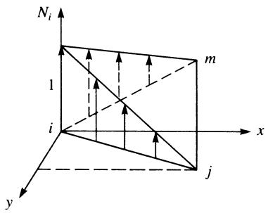(6.2.20) in abbreviated matrix form, we have $$ \{\psi \} = [ N ] \{d \} \tag {6.2.21} $$ where ½N is given by $$ [ N ] = \left[ \begin{array}{c c c c c c} N _ {i} & 0 & N _ {j} & 0 & N _ {m} & 0 \\ 0 & N _ {i} & 0 & N _ {j} & 0 & N _ {m} \end{array} \right] \tag {6.2.22} $$ We have now expressed the general displacements as functions of $\{ d \}$ , in terms of the shape functions $N _ { i } , N _ { j }$ , and $N _ { m }$ . The shape functions represent the shape of $\{ \psi \}$ when plotted over the surface of a typical element. For instance, $N _ { i }$ represents the shape of the variable u when plotted over the surface of the element for $u _ { i } = 1$ and all other degrees of freedom equal to zero; that is, $u _ { j } = u _ { m } = v _ { i } = v _ { j } = v _ { m } = 0$ . In addition, $u ( x _ { i } , y _ { i } )$ must be equal to $u _ { i } .$ Therefore, we must have $N _ { i } = 1 , N _ { j } = 0$ , and $N _ { m } = 0$ at $( x _ { i } , y _ { i } )$ . Similarly, $u ( x _ { j } , y _ { j } ) = u _ { j }$ . Therefore, $N _ { i } = 0 , \ N _ { j } = 1$ , and $N _ { m } = 0$ at $( x _ { j } , y _ { j } )$ . Figure 6–8 shows the shape variation of $N _ { i }$ plotted over the surface of a typical element. Note that $N _ { i }$ does not equal zero except along a line connecting and including nodes j and m. Finally, $N _ { i } + N _ { j } + N _ { m } = 1$ for all x and y locations on the surface of the element so that u and v will yield a constant value when rigid-body displacement occurs. The proof of this relationship follows that given for the bar element in Section 3.2 and is left as an exercise (Problem 6.1). The shape functions are also used to determine the body and surface forces at element nodes, as described in Section 6.3. 

text_image

N_i 1 i x y m j

Figure 6–8 Variation of $N _ { j }$ over the x-y surface of a typical element 

natural_image

Geometric shapes including a rectangle, a dashed rectangle, a hexagon, and a dashed-line square with x-y coordinate axes (no text or labels)

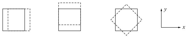
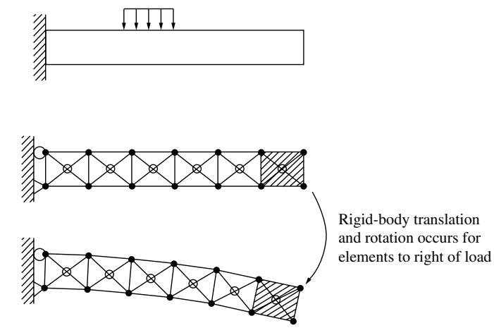
(a) Rigid-body modes of a plane stress element (from left to right, pure translation in x and y directions and pure rotation) 

text_image

Rigid-body translation and rotation occurs for elements to right of load

(b) Cantilever beam modeled using constant-strain triangle elements; elements to the right of the loading are stress-free Figure 6–9 Unstressed elements in a cantilever beam modeled with CST The requirement of completeness for the constant-strain triangle element used in a two-dimensional plane stress element is illustrated in Figure 6–9. The element must be able to translate uniformly in either the x or y direction in the plane and to rotate without straining as shown in Figure 6–9(a). The reason that the element must be able to translate as a rigid body and to rotate stress-free is illustrated in the example of a cantilever beam modeled with plane stress elements as shown in Figure 6–9(b). By simple statics, the beam elements beyond the loading are stressfree. Hence these elements must be free to translate and rotate without stretching or changing shape. # Step 3 Define the Strain= Displacement and Stress=Strain Relationships We express the element strains and stresses in terms of the unknown nodal displacements. # Element Strains The strains associated with the two-dimensional element are given by $$ \{\varepsilon \} = \left\{ \begin{array}{l} \varepsilon_ {x} \\ \varepsilon_ {y} \\ \gamma_ {x y} \end{array} \right\} = \left\{ \begin{array}{c} \frac {\partial u}{\partial x} \\ \frac {\partial v}{\partial y} \\ \frac {\partial u}{\partial y} + \frac {\partial v}{\partial x} \end{array} \right\} \tag {6.2.23} $$ Using Eqs. (6.2.19) for the displacements, we have $$ \frac {\partial u}{\partial x} = u _ {, x} = \frac {\partial}{\partial x} (N _ {i} u _ {i} + N _ {j} u _ {j} + N _ {m} u _ {m}) \tag {6.2.24} $$ or $u , \ j = N _ { i , x } u _ { i } + N _ { j , x } u _ { j } + N _ { m , x } u _ { m }$ ð6:2:25Þ where the comma followed by a variable indicates differentiation with respect to that variable. We have used $u _ { i , x } = 0$ because $u _ { i } = u ( x _ { i } , y _ { i } )$ is a constant value; similarly, $u _ { j , x } = 0$ and $u _ { m , x } = 0$ . Using Eqs. (6.2.18), we can evaluate the expressions for the derivatives of the shape functions in Eq. (6.2.25) as follows: $$ N _ {i, x} = \frac {1}{2 A} \frac {\partial}{\partial x} (\alpha_ {i} + \beta_ {i} x + \gamma_ {i} y) = \frac {\beta_ {i}}{2 A} \tag {6.2.26} $$ Similarly, $N _ { j , x } = \frac { \beta _ { j } } { 2 A } \qquad \mathrm { a n d } \qquad N _ { m , x } = \frac { \beta _ { m } } { 2 A }$ Nm; x ¼ bm ð6:2:27Þ Therefore, using Eqs. (6.2.26) and (6.2.27) in Eq. (6.2.25), we have $$ \frac {\partial u}{\partial x} = \frac {1}{2 A} (\beta_ {i} u _ {i} + \beta_ {j} u _ {j} + \beta_ {m} u _ {m}) \tag {6.2.28} $$ Similarly, we can obtain $$ \frac {\partial v}{\partial y} = \frac {1}{2 A} \left(\gamma_ {i} v _ {i} + \gamma_ {j} v _ {j} + \gamma_ {m} v _ {m}\right) \tag {6.2.29} $$ $$ \frac {\partial u}{\partial y} + \frac {\partial v}{\partial x} = \frac {1}{2 A} (\gamma_ {i} u _ {i} + \beta_ {i} v _ {i} + \gamma_ {j} u _ {j} + \beta_ {j} v _ {j} + \gamma_ {m} u _ {m} + \beta_ {m} v _ {m}) $$ Using Eqs. (6.2.28) and (6.2.29) in Eq. (6.2.23), we obtain $$ \{\varepsilon \} = \frac {1}{2 A} \left[ \begin{array}{c c c c c c} \beta_ {i} & 0 & \beta_ {j} & 0 & \beta_ {m} & 0 \\ 0 & \gamma_ {i} & 0 & \gamma_ {j} & 0 & \gamma_ {m} \\ \gamma_ {i} & \beta_ {i} & \gamma_ {j} & \beta_ {j} & \gamma_ {m} & \beta_ {m} \end{array} \right] \left\{ \begin{array}{l} u _ {i} \\ v _ {i} \\ u _ {j} \\ v _ {j} \\ u _ {m} \\ v _ {m} \end{array} \right\} \tag {6.2.30} $$ or $$ \{\varepsilon \} = [ \underline {{B}} _ {i} \quad \underline {{B}} _ {j} \quad \underline {{B}} _ {m} ] \left\{ \begin{array}{l} \underline {{d}} _ {i} \\ \underline {{d}} _ {j} \\ \underline {{d}} _ {m} \end{array} \right\} \tag {6.2.31} $$ where $$ [ B _ {i} ] = \frac {1}{2 A} \left[ \begin{array}{l l} \beta_ {i} & 0 \\ 0 & \gamma_ {i} \\ \gamma_ {i} & \beta_ {i} \end{array} \right] \quad [ B _ {j} ] = \frac {1}{2 A} \left[ \begin{array}{l l} \beta_ {j} & 0 \\ 0 & \gamma_ {j} \\ \gamma_ {j} & \beta_ {j} \end{array} \right] \quad [ B _ {m} ] = \frac {1}{2 A} \left[ \begin{array}{l l} \beta_ {m} & 0 \\ 0 & \gamma_ {m} \\ \gamma_ {m} & \beta_ {m} \end{array} \right] \tag {6.2.32} $$ Finally, in simplified matrix form, Eq. (6.2.31) can be written as $$ \{\varepsilon \} = [ B ] \{d \} \tag {6.2.33} $$ where $$ [ B ] = [ \underline {{B}} _ {i} \quad \underline {{B}} _ {j} \quad \underline {{B}} _ {m} ] \tag {6.2.34} $$ The B matrix is independent of the x and y coordinates. It depends solely on the element nodal coordinates, as seen from Eqs. (6.2.32) and (6.2.10). The strains in Eq. (6.2.33) will be constant; hence, the element is called a constant-strain triangle (CST). # Stress=Strain Relationship In general, the in-plane stress/strain relationship is given by $$ \left\{ \begin{array}{l} \sigma_ {x} \\ \sigma_ {y} \\ \tau_ {x y} \end{array} \right\} = [ D ] \left\{ \begin{array}{l} \varepsilon_ {x} \\ \varepsilon_ {y} \\ \gamma_ {x y} \end{array} \right\} \tag {6.2.35} $$ where ½D is given by Eq. (6.1.8) for plane stress problems and by Eq. (6.1.10) for plane strain problems. Using Eq. (6.2.33) in Eq. (6.2.35), we obtain the in-plane stresses in terms of the unknown nodal degrees of freedom as $$ \{\sigma \} = [ D ] [ B ] \{d \} \tag {6.2.36} $$ where the stresses fsg are also constant everywhere within the element. # Step 4 Derive the Element Stiffness Matrix and Equations Using the principle of minimum potential energy, we can generate the equations for a typical constant-strain triangular element. Keep in mind that for the basic plane stress element, the total potential energy is now a function of the nodal displacements $u _ { i } , v _ { i } , u _ { j } , \ldots , v _ { m }$ (that is, fdg) such that $$ \pi_ {p} = \pi_ {p} (u _ {i}, v _ {i}, u _ {j}, \dots , v _ {m}) \tag {6.2.37} $$ Here the total potential energy is given by $$ \pi_ {p} = U + \Omega_ {b} + \Omega_ {p} + \Omega_ {s} \tag {6.2.38} $$ where the strain energy is given by $$ U = \frac {1}{2} \iiint_ {V} \{\varepsilon \} ^ {T} \{\sigma \} d V \tag {6.2.39} $$ or, using Eq. (6.2.35), we have $$ U = \frac {1}{2} \iint_ {V} \{\varepsilon \} ^ {T} [ D ] \{\varepsilon \} d V \tag {6.2.40} $$ where we have used $\left[ D \right] ^ { T } = \left[ D \right]$ in Eq. (6.2.40). The potential energy of the body forces is given by $$ \Omega_ {b} = - \iint_ {V} \left\{\psi \right\} ^ {T} \{X \} d V \tag {6.2.41} $$ where $\{ \psi \}$ is again the general displacement function, and $\{ X \}$ is the body weight/ unit volume or weight density matrix (typically, in units of pounds per cubic inch or kilonewtons per cubic meter). The potential energy of concentrated loads is given by $$ \Omega_ {p} = - \{d \} ^ {T} \{P \} \tag {6.2.42} $$ where $\{ d \}$ represents the usual nodal displacements, and $\{ P \}$ now represents the concentrated external loads. The potential energy of distributed loads (or surface tractions) moving through respective surface displacements is given by $$ \Omega_ {s} = - \iint_ {S} \{\psi_ {S} \} ^ {T} \{T _ {S} \} d S \tag {6.2.43} $$ where $\{ T _ { S } \}$ represents the surface tractions (typically in units of pounds per square inch or kilonewtons per square meter), $\{ \psi _ { S } \}$ represents the field of surface displacements through which the surface tractions act, and S represents the surfaces over which the tractions $\{ T _ { S } \}$ act. Similar to $\operatorname { E q }$ . (6.2.21), we express $\{ \psi _ { S } \}$ as $\{ \psi _ { S } \} =$ $[ N _ { S } ] \{ d \}$ , where $[ N _ { S } ]$ represents the shape function matrix evaluated along the surface where the surface traction acts. Using Eq. (6.2.21) for $\{ \psi \}$ and Eq. (6.2.33) for the strains in Eqs. (6.2.40)– (6.2.43), we have $$ \begin{array}{l} \pi_ {p} = \frac {1}{2} \iint_ {V} \left\{d \right\} ^ {T} [ B ] ^ {T} [ D ] [ B ] \{d \} d V - \iint_ {V} \left\{d \right\} ^ {T} [ N ] ^ {T} \{X \} d V \\ - \{d \} ^ {T} \{P \} - \iint_ {S} \{d \} ^ {T} \left[ N _ {S} \right] ^ {T} \left\{T _ {S} \right\} d S \tag {6.2.44} \\ \end{array} $$ The nodal displacements fdg are independent of the general x-y coordinates, so fdg can be taken out of the integrals of Eq. (6.2.44). Therefore, $$ \begin{array}{l} \pi_ {p} = \frac {1}{2} \{d \} ^ {T} \iint_ {V} [ B ] ^ {T} [ D ] [ B ] d V \{d \} - \{d \} ^ {T} \iint_ {V} [ N ] ^ {T} \{X \} d V \\ - \{d \} ^ {T} \{P \} - \{d \} ^ {T} \iint_ {S} [ N _ {S} ] ^ {T} \{T _ {S} \} d S \tag {6.2.45} \\ \end{array} $$ From Eqs. (6.2.41)–(6.2.43) we can see that the last three terms of Eq. (6.2.45) represent the total load system f f g on an element; that is, $$ \{f \} = \iint_ {V} [ N ] ^ {T} \{X \} d V + \{P \} + \iint_ {S} [ N _ {S} ] ^ {T} \{T _ {S} \} d S \tag {6.2.46} $$ where the first, second, and third terms on the right side of Eq. (6.2.46) represent the body forces, the concentrated nodal forces, and the surface tractions, respectively. Using Eq. (6.2.46) in Eq. (6.2.45), we obtain $$ \pi_ {p} = \frac {1}{2} \{d \} ^ {T} \iiint_ {V} [ B ] ^ {T} [ D ] [ B ] d V \{d \} - \{d \} ^ {T} \{f \} \tag {6.2.47} $$ Taking the first variation, or equivalently, as shown in Chapters 2 and 3, the partial derivative of $\pi _ { p }$ with respect to the nodal displacements since $\pi _ { p } = \pi _ { p } ( \underline { { d } } )$ (as was previously done for the bar and beam elements in Chapters 3 and 4, respectively), we obtain $$ \frac {\partial \pi_ {p}}{\partial \{d \}} = \left[ \iiint_ {V} [ B ] ^ {T} [ D ] [ B ] d V \right] \{d \} - \{f \} = 0 \tag {6.2.48} $$ Rewriting Eq. (6.2.48), we have $$ \iint_ {V} [ B ] ^ {T} [ D ] [ B ] d V \{d \} = \{f \} \tag {6.2.49} $$ where the partial derivative with respect to matrix fdg was previously defined by Eq. (2.6.12). From Eq. (6.2.49) we can see that $$ [ k ] = \iint_ {V} [ B ] ^ {T} [ D ] [ B ] d V \tag {6.2.50} $$ For an element with constant thickness, t, Eq. (6.2.50) becomes $$ [ k ] = t \iint_ {A} [ B ] ^ {T} [ D ] [ B ] d x d y \tag {6.2.51} $$ where the integrand is not a function of x or y for the constant-strain triangular element and thus can be taken out of the integral to yield $$ [ k ] = t A [ B ] ^ {T} [ D ] [ B ] \tag {6.2.52} $$ where A is given by Eq. (6.2.9), ½B is given by Eq. (6.2.34), and ½D is given by Eq. (6.1.8) or Eq. (6.1.10). We will assume elements of constant thickness. (This assumption is convergent to the actual situation as the element size is decreased.) From Eq. (6.2.52) we see that $[ k ]$ is a function of the nodal coordinates (because ½B and A are defined in terms of them) and of the mechanical properties E and n (of which ½D is a function). The expansion of Eq. (6.2.52) for an element is $$ [ k ] = \left[ \begin{array}{l l l} {[ k _ {i i} ]} & {[ k _ {i j} ]} & {[ k _ {i m} ]} \\ {[ k _ {j i} ]} & {[ k _ {j j} ]} & {[ k _ {j m} ]} \\ {[ k _ {m i} ]} & {[ k _ {m j} ]} & {[ k _ {m m} ]} \end{array} \right] \tag {6.2.53} $$ where the $2 \times 2$ submatrices are given by $$ [ k _ {i i} ] = [ B _ {i} ] ^ {T} [ D ] [ B _ {i} ] t A $$ $$ [ k _ {i j} ] = [ B _ {i} ] ^ {T} [ D ] [ B _ {j} ] t A \tag {6.2.54} $$ $$ [ k _ {i m} ] = [ B _ {i} ] ^ {T} [ D ] [ B _ {m} ] t A $$ and so forth. In Eqs. (6.2.54), $[ B _ { i } ] , [ B _ { j } ]$ , and $\left[ B _ { m } \right]$ are defined by Eqs. (6.2.32). The ½k matrix is seen to be a $6 \times 6$ matrix (equal in order to the number of degrees of freedom per node, two, times the total number of nodes per element, three). In general, Eq. (6.2.46) must be used to evaluate the surface and body forces. When Eq. (6.2.46) is used to evaluate the surface and body forces, these forces are called consistent loads because they are derived from the consistent (energy) approach. For higher-order elements, typically with quadratic or cubic displacement functions, Eq. (6.2.46) should be used. However, for the CST element, the body and surface forces can be lumped at the nodes with equivalent results (this is illustrated in Section 6.3) and added to any concentrated nodal forces to obtain the element force matrix. The element equations are then given by $$ \left\{ \begin{array}{l} f _ {1 x} \\ f _ {1 y} \\ f _ {2 x} \\ f _ {2 y} \\ f _ {3 x} \\ f _ {3 y} \end{array} \right\} = \left[ \begin{array}{c c c c} k _ {1 1} & k _ {1 2} & \dots & k _ {1 6} \\ k _ {2 1} & k _ {2 2} & \dots & k _ {2 6} \\ \vdots & \vdots & & \vdots \\ k _ {6 1} & k _ {6 2} & \dots & k _ {6 6} \end{array} \right] \left\{ \begin{array}{l} u _ {1} \\ v _ {1} \\ u _ {2} \\ v _ {2} \\ u _ {3} \\ v _ {3} \end{array} \right\} \tag {6.2.55} $$ # Step 5 Assemble the Element Equations to Obtain the Global Equations and Introduce Boundary Conditions We obtain the global structure stiffness matrix and equations by using the direct stiffness method as $$ [ K ] = \sum_ {e = 1} ^ {N} [ k ^ {(e)} ] \tag {6.2.56} $$ and $$ \{F \} = [ K ] \{d \} \tag {6.2.57} $$ where, in Eq. (6.2.56), all element stiffness matrices are defined in terms of the global x-y coordinate system, fdg is now the total structure displacement matrix, and $$ \{F \} = \sum_ {e = 1} ^ {N} \{f ^ {(e)} \} \tag {6.2.58} $$ is the column of equivalent global nodal loads obtained by lumping body forces and distributed loads at the proper nodes (as well as including concentrated nodal loads) or by consistently using Eq. (6.2.46). (Further details regarding the treatment of body forces and surface tractions will be given in Section 6.3.) In the formulation of the element stiffness matrix Eq. (6.2.52), the matrix has been derived for a general orientation in global coordinates. Equation (6.2.52) then applies for all elements. All element matrices are expressed in the global-coordinate orientation. Therefore, no transformation from local to global equations is necessary. However, for completeness, we will now describe the method to use if the local axes for the constant-strain triangular element are not parallel to the global axes for the whole structure. 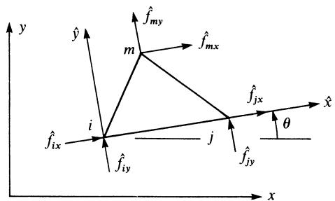If the local axes for the constant-strain triangular element are not parallel to the global axes for the whole structure, we must apply rotation-of-axes transformations similar to those introduced in Chapter 3 by Eq. (3.3.16) to the element stiffness matrix, as well as to the element nodal force and displacement matrices. We illustrate the transformation of axes for the triangular element shown in Figure 6–10, considering the element to have local axes x^-y^ not parallel to global axes x-y. Local nodal forces are shown in the figure. The transformation from local to global equations follows the procedure outlined in Section 3.4. We have the same general expressions, Eqs. (3.4.14), (3.4.16), and (3.4.22), to relate local to global displacements, forces, and stiffness matrices, respectively; that is, $$ \underline {{{\hat {d}}}} = \underline {{{T}}} \underline {{{d}}} \quad \underline {{{\hat {f}}}} = \underline {{{T}}} \underline {{{f}}} \quad \underline {{{k}}} = \underline {{{T}}} ^ {T} \underline {{{\hat {k}}}} \underline {{{T}}} \tag {6.2.59} $$ where Eq. (3.4.15) for the transformation matrix T used in Eqs. (6.2.59) must be expanded because two additional degrees of freedom are present in the constant-strain 

text_image

y ŷ m f̂_my f̂_mx i f̂_ix f̂_iy j f̂_jx θ f̂_jy x

Figure 6–10 Triangular element with local axes not parallel to global axes triangular element. Thus, Eq. (3.4.15) is expanded to $$ \underline {{T}} = \left[ \begin{array}{c c c c c c} C & S & 0 & 0 & 0 & 0 \\ - S & C & 0 & 0 & 0 & 0 \\ \hline 0 & 0 & C & S & 0 & 0 \\ 0 & 0 & - S & C & 0 & 0 \\ \hline 0 & 0 & 0 & 0 & C & S \\ 0 & 0 & 0 & 0 & - S & C \end{array} \right] \begin{array}{l} u _ {i} \\ v _ {i} \\ u _ {j} \\ v _ {j} \\ u _ {m} \\ v _ {m} \end{array} \tag {6.2.60} $$ where C ¼ cos y, S ¼ sin y, and y is shown in Figure 6–10. # Step 6 Solve for the Nodal Displacements We determine the unknown global structure nodal displacements by solving the system of algebraic equations given by Eq. (6.2.57). # Step 7 Solve for the Element Forces (Stresses) Having solved for the nodal displacements, we obtain the strains and stresses in the global x and y directions in the elements by using Eqs. (6.2.33) and (6.2.36). Finally, we determine the maximum and minimum in-plane principal stresses $\sigma _ { 1 }$ and $\sigma _ { 2 }$ by using the transformation Eqs. (6.1.2), where these stresses are usually assumed to act at the centroid of the element. The angle that one of the principal stresses makes with the x axis is given by Eq. (6.1.3). # Example 6.1 Evaluate the stiffness matrix for the element shown in Figure 6–11. The coordinates are shown in units of inches. Assume plane stress conditions. Let $E = 3 0 \times 1 0 ^ { 6 }$ psi, $\nu = 0 . 2 5 ,$ , and thickness $t = 1$ in. Assume the element nodal displacements have been determined to be $u _ { 1 } = 0 . 0 , v _ { 1 } = 0 . 0 0 2 5$ in., $u _ { 2 } = 0 . 0 0 1 2$ in., $v _ { 2 } = 0 . 0 , u _ { 3 } = 0 . 0$ , and $v _ { 3 } = 0 . 0 0 2 5$ in. Determine the element stresses. 

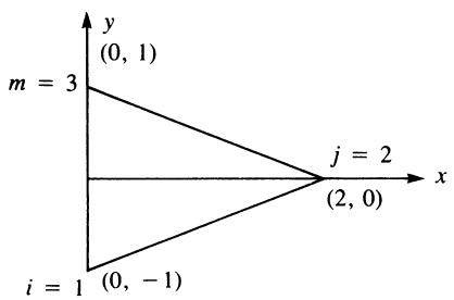
text_image

m = 3 (0, 1) j = 2 (2, 0) x i = 1 (0, -1)

Figure 6–11 Plane stress element for stiffness matrix evaluation