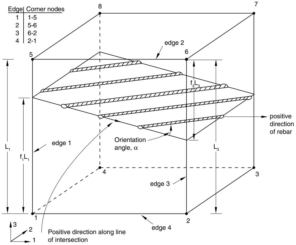
Figure 2.2.4–13 Element with two layers of isoparametric rebar. 

text_image

Edge| Corner nodes 1 1-5 2 5-6 3 6-2 4 2-1 8 7 5 6 f₃L₃ L₁ f₁L₁ edge 1 Orientation angle, α 4 L₃ positive direction of rebar 3 2 1 edge 3 edge 4 1 2 3 Positive direction along line of intersection

Figure 2.2.4–14 Orientation example for three-dimensional skew rebar modeling, isoparametric direction 2. Shown in the mapped isoparametric element. Example: isoparametric rebar For example, the following input defines the isoparametric rebar shown in Figure 2.2.4–13: \*HEADING ISOPARAMETRIC REBAR \*NODE 2, 10., 0. 3, 10., 5. 6, 10., 0., 12.5 7, 10., 5., 12.5 8, 0., 5., 7.5 ```csv * ELEMENT, TYPE=C3D8R, ELSET=ONE 1,1,2,3,4,5,6,7,8 * REBAR, ELEMENT=CONTINUUM, MATERIAL=STEEL, GEOMETRY=ISOPARAMETRIC, NAME=LAYER_A ONE,.04,2.5,49.32628,0.25,4,2 * REBAR, ELEMENT=CONTINUUM, MATERIAL=STEEL, GEOMETRY=ISOPARAMETRIC, NAME=LAYER_B ONE,.04,1.,63.43494,0.5,3,2 *MATERIAL, NAME=STEEL * ELASTIC 30.E6, ... 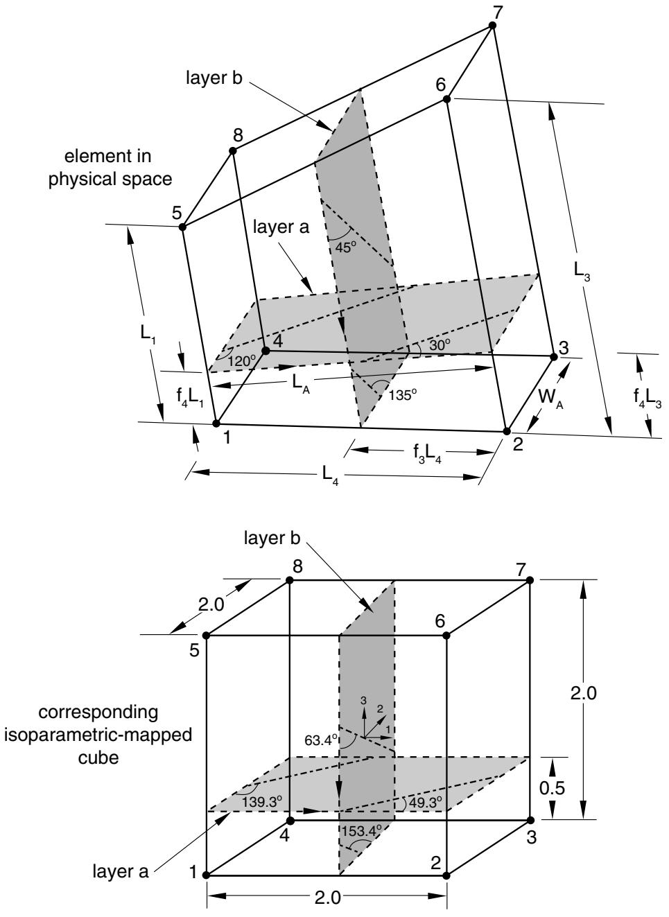``` Rebar layers A and B are defined using isoparametric direction 2. From Figure 2.2.4–12 the position of the layers must be given with respect to the face with nodes 1-5-6-2. The fractional distance defining the position of intersection of layer A with this face can be measured from edge 4 (edge with nodes 2–1) along edge 3 (edge with nodes 6–2), as shown in Figure 2.2.4–13. For layer $A , f _ { 4 } = . 2 5$ . It could also be given from edge 2 (edge with nodes 5–6), so that $f _ { 2 } = 1 . 0 - f _ { 4 } = . 7 5$ . The orientation of rebar for layer A in physical space is defined by an angle, $\beta ,$ equal to $3 0 ^ { \circ }$ for layer A. This angle must be transformed into the corresponding angle in the isoparametric-mapped cube. This transformation can be done as follows: consider a single rebar that intersects the intersecting line (described above) and an adjacent edge (see Figure 2.2.4–15). 

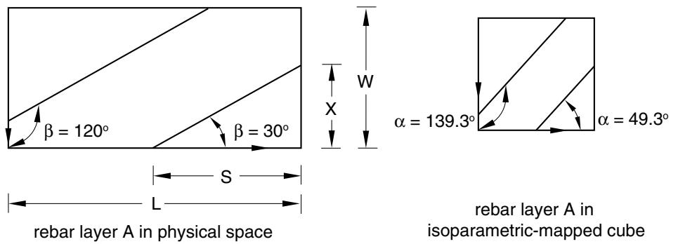
text_image

β = 120° β = 30° S L rebar layer A in physical space W X α = 139.3° α = 49.3° rebar layer A in isoparametric-mapped cube

Figure 2.2.4–15 Example defining isoparametric rebar. From the figure $\beta = X / S$ . The length of the rebar layer along the intersecting line is $L ,$ and the length of the opposite edge is W. Consider the same rebar in the rebar layer in the isoparametric-mapped cube. The orientation angle, , is given by $\alpha = x / s ,$ , where $x = 2 X / W$ and $s = 2 S / L$ . (The 2 is included because the isoparametric-mapped cube is a $2 \times 2 \times 2$ cube.) This expression can be simplified to give $$ \tan \alpha = \frac {X}{W} \frac {L}{S} = \frac {L}{W} \tan \beta . $$ For layer A, , , $\beta = 3 0 ^ { \circ }$ , and $\alpha = 4 9 . 3 3 ^ { \circ }$ , where is the orientation angle that must be specified. The fractional distance defining the position of the intersection of layer B with this face can be measured from edge 3 (edge with nodes 6–2); $f _ { 3 } = . 5$ . It could also be measured from edge 1 (edge with nodes 1–5), such that $f _ { 1 } = 1 . 0 - f _ { 3 }$ . The orientation angle for layer B in the rebar layer is $4 5 ^ { \circ }$ . In the isoparametric-mapped cube $L = 1 0$ , , , and $\alpha = 6 3 . 4 3 ^ { \circ }$ . Since an isoparametric rebar layer always lies in two of the isoparametric directions, an alternative but equivalent definition can be given. For example, layer A also lies in isoparametric direction 1, with the intersecting face having nodes 1-4-8-5. The fractional distance for layer A, measured from edge 1 (edge with nodes 1–4), is $f _ { 1 } = . 2 5$ . The positive sense of the line of intersection is from edge 2 (edge with nodes 4–8) to edge 4 (edge with nodes 5–1); therefore, , , $W = 1 0 . 0 7 7$ , and $\alpha = 1 3 9 . 3 2 ^ { \circ }$ . Layer B also lies in isoparametric direction 3, with the intersecting face having nodes 1-2-3-4. The fractional distance for layer B, measured from edge 2 (edge with nodes 2–3), is $f _ { 2 } = . 5$ . The positive sense of the intersecting line is from edge 1 (edge with nodes 1–2) to edge 3 (edge with nodes 3–4); therefore, the orientation angle of the rebar in physical space is , , , and in the isoparametric-mapped cube $\alpha = 1 5 3 . 4 3 ^ { \circ }$ . # Defining skew rebars You specify the elements that contain the rebars; the cross-sectional area, A, of each rebar; the rebar spacing, s; the rebar orientation, (as described above); and the isoparametric direction. In addition, you specify the fractional distance f along the element edge for each edge of the intersecting face defined in Figure 2.2.4–12. Only the values corresponding to the two edges that the rebar intersects can be nonzero. Input File Usage: Use the following option to define layers of skew rebars in three-dimensional continuum elements: $\scriptstyle * { \mathrm { R E B A R , ~ E L E M E N T } } = \scriptstyle { \mathrm { C O N T I N U U M , ~ M A T E R I A L } } = m a t ,$ # Example: skew rebar For example, the following input defines the skew rebar shown in Figure 2.2.4–16:

*HEADING
*NODE
1,	0.,	0.
2,	10.,	0.
3,	10.,	5.
4,	0.,	5.
5,	0.,	0.,	7.5
6,	10.,	0.,	12.5
7,	10.,	5.,	12.5
8,	0.,	5.,	7.5


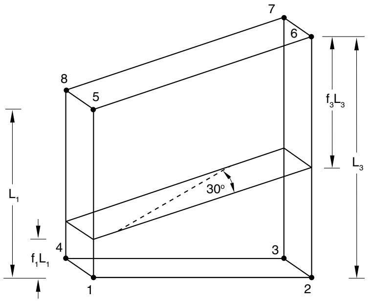
text_image

L₁ f₁L₁ 1 2 3 4 5 6 7 30° f₃L₃ L₃

Figure 2.2.4–16 Example defining skew rebar. ```txt * ELEMENT, TYPE=C3D8R, ELSET=ONE 1,1,2,3,4,5,6,7,8 * REBAR, ELEMENT=CONTINUUM, MATERIAL=STEEL, GEOMETRY=SKEW, NAME=LAYER_A ONE, .04, 2.5, 55.28, , 2 .2, 0., .4, .0 *MATERIAL, NAME=STEEL * ELASTIC 30.E6, ... ``` The rebar layer is defined using isoparametric direction 2. The intersecting face is defined in Figure 2.2.4–12 and has nodes 1-5-6-2. The position of the rebar layer is given by its intersection with the edges of this face; the fractional distances, $f _ { 1 }$ and $f _ { 3 } ,$ , are shown in Figure 2.2.4–16. The orientation angle $\beta$ of the rebar in physical space is 30°. Following the same procedure for calculating as was described for isoparametric rebar, , , and the orientation angle in the isoparametric-mapped cube is 55.28°. # Defining single rebars in three-dimensional continuum elements You can define single rebars in three-dimensional continuum elements; in this case the rebar is assumed to be placed along one of the element’s isoparametric directions. The rebar is then located by its intersection with the intersecting face (defined in Figure 2.2.4–12). The intersections of constant isoparametric lines with edges 1 and 2 of the intersecting face are given by fractional distances along edges 1 and 2, measured from the first node of each edge, as shown in Figure 2.2.4–11. You specify the elements that contain the rebars; the cross-sectional area, A, of each rebar; the fractional distances locating the rebar’s position in the element, $f _ { 1 }$ and $f _ { 2 } ;$ and the isoparametric direction. Give the fractional distances with respect to edge 1 and edge 2 for the isoparametric direction chosen, as defined in Figure 2.2.4–12. # Input File Usage: Use the following option to define single rebars in three-dimensional continuum elements: \*REBAR, ELEMENT=CONTINUUM, MATERIAL=mat, SINGLE # Defining the rebar material The material properties of the rebars are distinct from those of the underlying element and are defined by a separate material definition (“Material data definition,” Section 21.1.2). You must associate each rebar definition with a set of material properties. The following material behavior cannot be used in Abaqus/Standard to define rebar materials: • “Porous metal plasticity,” Section 23.2.9. The following material behaviors cannot be used in Abaqus/Explicit to define rebar materials: • “Defining fully anisotropic elasticity” in “Linear elastic behavior,” Section 22.2.1; • “Defining orthotropic elasticity by specifying the terms in the elastic stiffness matrix” in “Linear elastic behavior,” Section 22.2.1; • “Equation of state,” Section 25.2.1; • “Anisotropic yield/creep,” Section 23.2.6; • “Porous metal plasticity,” Section 23.2.9; • “Extended Drucker-Prager models,” Section 23.3.1; • “Modified Drucker-Prager/Cap model,” Section 23.3.2; • “Crushable foam plasticity models,” Section 23.3.5; or • “Cracking model for concrete,” Section 23.6.2. Although Abaqus/Standard will allow for a rebar material to be defined with orthotropic elasticity (“Defining orthotropic elasticity by specifying the terms in the elastic stiffness matrix” in “Linear elastic behavior,” Section 22.2.1) or anisotropic elasticity (“Defining fully anisotropic elasticity” in “Linear elastic behavior,” Section 22.2.1), $D _ { 1 1 1 1 }$ is the only meaningful material constant in these definitions. $D _ { 1 1 1 1 }$ is used to compute the strain in the rebar direction, $\varepsilon _ { 1 1 }$ , using the corresponding stress component, $\sigma _ { 1 1 }$ , as discussed in “Linear elastic behavior,” Section 22.2.1; no other strain or stress components exist in rebars. In Abaqus/Standard density is ignored for the rebar material properties. Hence, the mass of the rebar is neglected in eigenvalue extraction and implicit dynamic procedures and for gravity, centrifugal, and rotary acceleration distributed loads. Input File Usage: Use the following option to associate a material definition with a rebar definition: \*REBAR, ELEMENT=elem, MATERIAL=mat # Initial conditions Initial conditions (“Initial conditions in Abaqus/Standard and Abaqus/Explicit,” Section 34.2.1) can be used to define rebar prestress or solution-dependent values for rebars. # Defining prestress in rebar For structures in which reinforcing is defined (such as reinforced concrete structures), you can use initial conditions to define the prestress in the rebars. In such cases in Abaqus/Standard the structure must be brought to a state of equilibrium before it is actively loaded by means of an initial static analysis step (“Static stress analysis,” Section 6.2.2) with no external loads applied (or, perhaps, with the “dead” loads only)—see “Defining initial stresses” in “Initial conditions in Abaqus/Standard and Abaqus/Explicit,” Section 34.2.1. Input File Usage: \*INITIAL CONDITIONS, TYPE=STRESS, REBAR element number or element set name, rebar name, prestress value # Holding prestress in rebar in Abaqus/Standard If prestress is defined in the rebars and unless the prestress is held fixed, it will be allowed to change during an equilibrating static analysis step; this is a result of the straining of the structure as the selfequilibrating stress state establishes itself. An example is the pretension type of concrete prestressing in which reinforcing tendons are initially stretched to a desired tension before being covered by concrete. After the concrete cures and bonds to the rebar, release of the initial rebar tension transfers load to the concrete, introducing compressive stresses in the concrete. The resulting deformation in the concrete reduces the stress in the rebar. Alternatively, you can keep the initial stress defined in some or all of the rebars constant during this initial equilibrium solution. An example is the post-tension type of concrete prestressing; the rebars are allowed to slide through the concrete (normally they are in conduits), and the prestress loading is maintained by some external source (prestressing jacks). The magnitude of the prestress in the rebar is normally part of the design requirements and must not be reduced as the concrete compresses under the loading of the prestressing. Normally, the prestress is held constant only in the first step of an analysis. This is generally the more common assumption for prestressing. If the prestress is not held constant in analysis steps following the step in which it is held constant, the stress in the rebar will change due to additional deformation in the concrete. If there is no additional deformation, the stress in the rebar will remain at the level set by the initial conditions. If the loading history is such that no plastic deformation is induced in the concrete or rebar in steps subsequent to the steps in which the prestress is held constant, the stress in the rebar will return to the level set by the initial conditions upon removal of the loading applied in those steps. Input File Usage: \*PRESTRESS HOLD # Defining the initial values of solution-dependent state variables for rebars You can define the initial values of solution-dependent state variables for rebars within elements. See “Initial conditions in Abaqus/Standard and Abaqus/Explicit,” Section 34.2.1, for details. Input File Usage: \*INITIAL CONDITIONS, TYPE=SOLUTION, REBAR # Output Rebar force output is available at the rebar integration locations with output variable RBFOR. The rebar force is equal to the rebar stress times the current rebar cross-sectional area. The current cross-sectional area of the rebar is calculated by assuming the rebar is made of an incompressible material, regardless of the actual material definition. For rebars in membrane or shell elements output variables RBANG and RBROT identify the current orientation of isoparametric or skew rebar within the element and the relative rotation of the rebar as a result of finite deformation, respectively. These quantities are measured with respect to the user-specified isoparametric direction in the element, not the default local element system or the orientation-defined system. See “Rebar modeling in shell, membrane, and surface elements,” Section 3.7.3 of the Abaqus Theory Guide. See “Abaqus/Standard output variable identifiers,” Section 4.2.1, and “Abaqus/Explicit output variable identifiers,” Section 4.2.2, for information on additional output quantities such as stress and strain. For rebars in membrane or shell elements with multiple integration points, output quantities are available at the integration points and at the centroid of the element. # Specifying the direction for rebar angle output in shell and membrane elements The output quantities RBANG and RBROT can be measured from either of the isoparametric directions in the plane of the shell or the membrane. You can specify the desired isoparametric direction from which the rebar angle will be measured (1 or 2). In axisymmetric shells and membranes the first isoparametric direction coincides with the meridional direction, and the second isoparametric direction coincides with the hoop direction. The rebar angle is measured from the isoparametric direction to the rebar with a positive angle defined as a counterclockwise rotation around the element’s normal direction. The default direction is the first isoparametric direction. 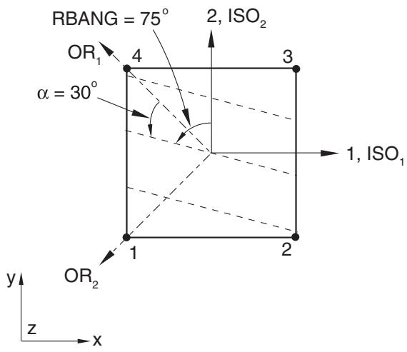Input File Usage: Use any of the following options: *REBAR, ELEMENT=SHELL, MATERIAL=mat, ISODIRECTION=n *REBAR, ELEMENT=AXISHELL, MATERIAL=mat, ISODIRECTION=n *REBAR, ELEMENT=MEMBRANE, MATERIAL=mat, ISODIRECTION=n *REBAR, ELEMENT=AXIMEMBRANE, MATERIAL=mat, ISODIRECTION=n # Example As an example, a user-defined local coordinate system is used to define skewed rebar in a shell element (skew angle $\alpha = 3 0 ^ { \circ } )$ , and the output value of RBANG is $7 5 ^ { \circ }$ , as illustrated in Figure 2.2.4–17: 

text_image

RBANG = 75° 2, ISO₂ OR₁ 4 α = 30° 3 1, ISO₁ 1 2 y z x

ISO = isoparametric directions OR = user-defined local directions 1, 2 = default local directions Figure 2.2.4–17 RBANG measurement for skew rebar defined relative to user-defined local coordinate directions. ```txt *REBAR, ELEMENT=SHELL, MATERIAL=MAT1, NAME=REBARB, GEOMETRY=SKEW, ORIENTATION=ORIENT, ISODIRECTION=2 ELSET1, 0.01, 0.1, 0.0, 30. *ORIENTATION, SYSTEM=RECTANGULAR, NAME=ORIENT -0.7071, 0.7071, 0.0, -0.7071, -0.7071, 0.0 3, 0.0 ``` The rebars are located at the midsurface of the shell. Output variable RBANG is measured from the second isoparametric direction to the rebar. If the first isoparametric direction were chosen instead, output variable RBANG would report an angle of 165°. # Visualizing rebar orientation and results in rebar Abaqus/CAE does not support visualization of element-based rebar or rebar results. Abaqus/CAE does support visualization of rebar defined as described in “Defining reinforcement,” Section 2.2.3.